TrialComputeMove

class TrialComputeMove : public feasst::TrialCompute

Move a selection of particles and sites.

Derivation of the acceptance criteria follows Lecture 9 of Prof. David Kofke’s Molecular Simulation course CE 530.

http://www.eng.buffalo.edu/~kofke/ce530/Lectures/lectures.html

For this type of move, the potential energy of the system, U, is the only thermodynamic variable which changes. Thus, whether in the canonical ensemble or otherwise, the probability distribution,

\(\pi_i \propto \exp(-\beta U_i)\)

because the other thermodynamic variables such as number of particles, or volume do not change.

The following table describes the transition probabilities associated with the chosen trial move, and its reverse trial that is considered for the purpose of satisfying detailed balance. Thus, the probability shown represents the probability of transitioning from the old to the new state, \(\pi_{on}\). And the reverse transition probability is from new to old, \(\pi_{no}\).

Forward event [reverse event]	Probability, \(\pi_{on}\) [reverse probability, \(\pi_{no}\)]
Select particle of type t [Select particle of type t]	\(1/N_t\) \([1/N_t]\)
Move to new position [Move to old position]	\(1/v\) \([1/v]\)
Accept [Accept]	\(\min(1, \chi)\) \([\min(1, 1/\chi)]\)

where \(\chi\) is the acceptance probability that we can now derive by imposing the (local) detailed balance condition.

For (local) detailed balance, the probability of being in the old state, \(\pi_o\), times the probability of transitioning from the old to the new state, \(\pi_{on}\), should be equal to the probability of being in the new state, \(\pi_n\) times the probability of transitioning from the new to old state, \(\pi_{no}\).

\(\pi_o \pi_{on} = \pi_n \pi_{no}\)

Substituting the probability distribution and transition probabilities yields

\(\frac{\min(1, \chi)\exp(-\beta U_o)}{N_t v} = \frac{\min(1, 1/\chi)\exp(-\beta U_n)}{N_t v}\)

\(\frac{\min(1, \chi)}{\min(1, 1/\chi)} = \exp[-\beta(U_n - U_o)] = \exp(-\beta\Delta U)\)

The left hand side is \(\chi\) for both cases of \(\chi <= 1\) and \(\chi > 1\). Thus,

\(\chi = \exp(-\beta\Delta U)\)

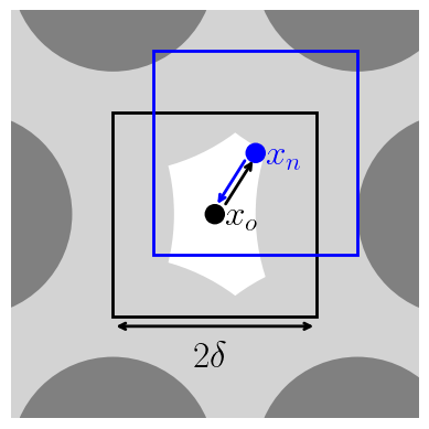
For configurational bias, consider multiple trial positions and select one. This can lead to higher acceptance probability or larger displacements, \(\delta\), in each of D dimensions. It is also parallelizable (https://doi.org/10.1103/PhysRevE.51.1560) and allows the use of dual-cut CB (https://doi.org/10.1080/002689798167881).

Forward event [reverse event]	Probability, \(\pi_{on}\) [reverse probability, \(\pi_{no}\)]
Select particle of type t [Select particle of type t]	\(1/N_t\) \([1/N_t]\)
Generate k positions about \(x_o\). Probability \(x_n\) is in k. [Generate j positions about \(x_n\). Probability \(x_o\) is in j.]	\(k/\delta^D\) \([j/\delta^D]\)
Pick \(x_n\) in k positions. [Pick \(x_o\) in j positions.]	\(P_k\) \(P_j\)
Accept [Accept]	\(\min(1, \chi)\) \([\min(1, 1/\chi)]\)

Applying (local) detailed balance yields

\(\chi = \frac{P_j}{P_k} \exp[-\beta(U_n - U_o)]\)

Note that the number of new and old positions must be equal, \(j = k\). In this case, the j and k indices are retained to distinguish between positions generated about the old or new position.

If the probability of picking a position is chosen as the typical Rosenbluth factor,

\(P_m = \exp(-\beta U)/\sum_i^m \exp(-\beta U_i)\).

Thus, the acceptance is given by

\(\chi = \frac{\sum_i^k \exp(-\beta U_i)}{\exp(-\beta U_n)}\frac{\exp(-\beta U_o)}{\sum_i^j \exp(-\beta U_i)}\exp(-\beta(U_n - U_o))\)

\(\chi = \frac{\sum_i^k \exp(-\beta U_i)}{\sum_i^j \exp(-\beta U_i)}\).

Note that the sum over j is for randomly generated positions within \(\delta\) of the new position, while the sum over k is for randomly generated positions within \(\delta\) of the old position. This means that the sum over j includes the old position.

For dual-cut configurational bias, the new trials are instead chosen from a reference potential, \(U^r\), that is ideally much faster to compute than the full potential but still contains sampling-relevant terms (e.g., excluded volume in a dense system).

\(P_m(U) = \exp(-\beta U^r)/\sum_i^m \exp(-\beta U_i^r)\)

\(\chi = \frac{\sum_i^k \exp(-\beta U^r_i)}{\sum_i^j \exp(-\beta U_i^r)}\exp\{-\beta[(U_n-U_n^r) - (U_o-U_o^r)]\}\)

Note that these equations consider only a single-site particle.

Subclassed by feasst::ComputeAVB2, feasst::ComputeAVB4

Public Functions

void perturb_and_acceptance(Criteria *criteria, System *system, Acceptance *acceptance, std::vector<TrialStage*> *stages, Random *random)

Perform the Perturbations and determine acceptance.