12. Addons¶

The output of MOSAIC is often processed further to generate plots or performe more sophisticated analysis. We facilitate this process by providing addon packages that make it easy to import the SQLite database generated by a MOSAIC analysis into Mathematica, Matlab or IGOR. The interfaces for these programs are described in more detail in this section.

12.1. Mathematica¶

12.1.1. Installation¶

The analysis output generated by MOSAIC can be imported into Mathematica for further processing. This accomplished with two packages: the low level MosaicUtils and MosaicAnalysis, which contains additional analysis routines. The addon package must first be installed to one of the locations in the Mathematica path. Alternatively, the required package files can be installed to the Applications folder using setuptools on Mac OS X and Linux by issuing the command below in the root folder of the MOSAIC code. Instructions for installing the package files for Windows are available here.

python setup.py mosaic_addons --mathematica

12.1.2. MosaicUtils¶

MosaicUtils provides low level functions to interact with a database output by MOSAIC. MosaicUtils can use a native Mathematica (slower, default) or Python (faster, but experimental) backend to query databases output by MOSAIC.

Note

To select the Python backend, please call the SetQueryBackend function as described below. If you use a virtual environment with Python, please call the SetVirtualEnv function after you install this addon.

SetQueryBackend[backend]

Args:

backend : select the Mathematica (default) or Python (faster, experimental) backend to run SQLite queries.

Returns:

None

ReadQueryBackend[]

Args:

None

Returns:

The backend used to run SQLite queries.

SetVirtualEnv[virtualenv]

Args:

virtualenv : name of the virtual environment configured for use with MOSAIC

Returns:

None

PrintMDKeys[dbfile]

Returns a list of column headings from the metadata table.

Args:

dbfile : full path to the database file

Returns:

A list of column names in the table metadata.

PrintMDTypes[dbfile]

Returns a list of column types from the metadata table.

Args:

dbfile : full path to the database file

Returns:

A list of column types in the table metadata.

QueryDB[dbfile, query]

Queries the metadata table using the supplied SQL query.

Args:

dbfile : full path to the database file
query : a SQL query

Returns:

A nested list of query results.

PlotEvents[dbfile, FsKHz, nEvents]

Plot the event-time series if stored in the database (see the Settings File section for details on saving time-series to the analysis output).

Args:

dbfile : full path to the database file
FsKHz : sampling frequency in kHz.
nEvents : (optional) limit the plot to the first n entries in the database

Returns:

A dynamic object that allows the user to browse event time-series and fits.

GetAnalysisAlgorithm[db]

Returns the analysis algorithm used to process the current data set.

Args:

db : full path to a database file

Returns:

Algorithm used to analyze data.

MosaicUtils Examples

Once installed as described above, MosaicUtils must be imported as shown below.

In[1]= <<MosaicUtils`

SQL queries require the exact column names when querying data from a table (see Database Structure and Query Syntax). Column names in the metadata table, which stores the main results from the analaysis can be retrieved using the PrintMDKeys function as shown below. In this example, the column names returned correspond to an analysis performed using the adept2State algorithm.

In[2]= PrintMDKeys["<mosaicroot>/data/eventMD-PEG29-Reference.sqlite"]

Out[2]= {"recIDX", "ProcessingStatus", "OpenChCurrent",
        "BlockedCurrent", "EventStart", "EventEnd",
        "BlockDepth", "ResTime", "RCConstant", "AbsEventStart",
        "ReducedChiSquared", "TimeSeries"
        }

The MosaicUtils package allows the output of MOSAIC to be queried just like from Python. This accomplished using the QueryDB function. In the example below, we retrieve a column that returns the start time of the first 10 entries in the metadata table that have their ProcessingStatus set to normal. The results are then returned in a standard list. Note that QueryDB accepts a standard SQL query as described in more detail in the Database Structure and Query Syntax section.

In[3]= QueryDB[
        "<mosaicroot>/data/eventMD-PEG29-Reference.sqlite",
        "select AbsEventStart from metadata where ProcessingStatus='normal' limit 10"
        ]

Out[3]= {
        {1.84376}, {4.54439}, {5.26933}, {6.01253}, {6.80369},
        {8.48988}, {10.841}, {11.2246}, {13.2892}, {16.3983}
        }

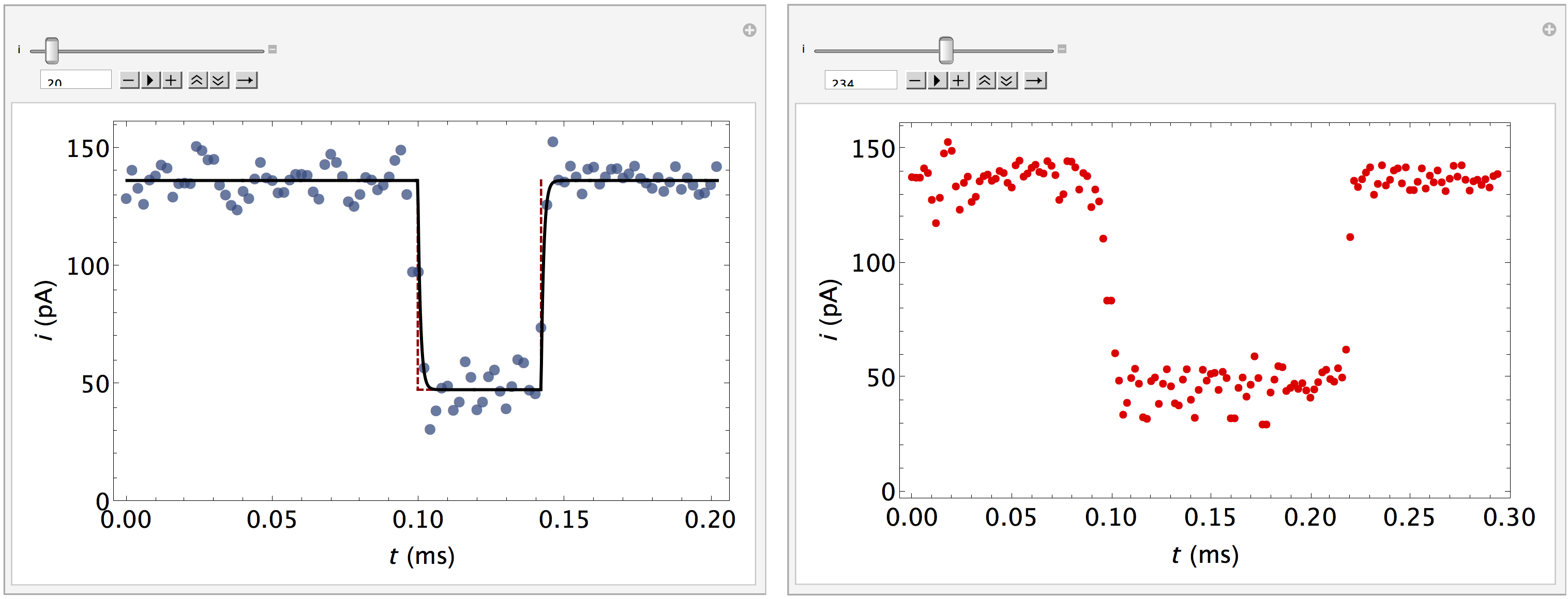
Finally, the addon package allows us to plot individual events if time-series data was stored in the database. This is accomplished using the PlotEvents function, and provides a convenient tool to visually inspect the output of a MOSAIC analysis. In the example below, we inspect the events stored in the reference PEG28 data set included with MOSAIC. PlotEvents returns a dynamic object that allows the user to inspect all the events in a database. An event that was properly characterized by the code is plotted with blue markers (left). The plot is overlaid with the optimized fit function (black) and an idealized pulse (red dashed). Events that were not properly fit are plotted with red markers (right).

In[4]= PlotEvents["<mosaicroot>/data/eventMD-PEG29-Reference.sqlite", 500]

12.1.3. MosaicAnalysis¶

MosaicAnalysis builds on the MosaicUtils package and provides basic analysis functions such as estimating the capture rate of molecules partitioning into a channel, or the mean residence time. Additionally, new functionality can be created by combining the functions defined below.

ScaledSingleExponentialFit[hist, lambda, lambda0]

Scale the histogram with the number of counts in the first bin. Fit a single exponential of the form a exp(-t/tau) to the scaled histogram.

Args:

hist : a histogram with format {{bin1, counts1}, {bin2, counts2}, …, {binN,countsN}}
lambda : parameter of the distribution. This symbol must be passed from the calling function.
lambda0 : initial guess for lambda.

PlotScaledSingleExponentialFit[hist, ftfunc, plotopts]

Args:

hist : a histogram with format {{bin1, counts1}, {bin2, counts2}, …, {binN,countsN}}
ftfunc : an optimized fit, defined as a virtual function.
plotopts: a list of options to control the plot output.

CaptureRate[arrtimes, stime, etime, nbins, plotopts]

Estimate the capture rate of molecules by a channel by analyzing the arrival times of individual molecules. The arrival times of a stochastic process follow a single exponential distribution. This function first calculate a histogram of arrival times and then fits a single exponential function to the data.

Args:

arrtimes : a list of absolute start times (AbsEventStart) queried from a database.
stime : lower limit of the arrival times distribution
etime : upper limit of the arrival times distribution
nbins : number of bins
plotopts : a list of options to control the plot output.

Returns:

The mean capture rate, a plot of the underlying distribution of arrival times, the arrival times distribution and the optimized fit function.

ArrivalTimes[abseventstart]

Calculate the arrival times from a list of the absolute start time of each event in a data set.

Args:

abseventstart : a list of absolute start times (AbsEventStart) queried from a database.

Returns:

A list of arrival times.

MosaicAnalysis Examples

In[1]= <<MosaicUtils`
In[2]= <<MosaicAnalysis`

In the following example, we estimate the capture rate of PEG28 from the reference data set included with the MOSAIC source. The first argument fo CaptureRate is a list of the absolute start time of each event in the database. This data can be obtained using the query shown below. The remaining arguments to CaptureRate define the parameters of the arrival times distribution, the lower and upper limit of the arrival times and the number of bins. The function returns the mean capture rate and standard error, a plot that shows the underlying arrival times distribution, raw data used to generate the capture rate histogram, and a pure best-fit function.

In[3]= CaptureRate[
        QueryDB[
        "<mosaicroot>/data/eventMD-PEG29-Reference.sqlite",
        "select AbsEventStart from metadata where
                ProcessingStatus='normal' and ResTime > 0.01"
        ], 0.0, 0.05, 50
]

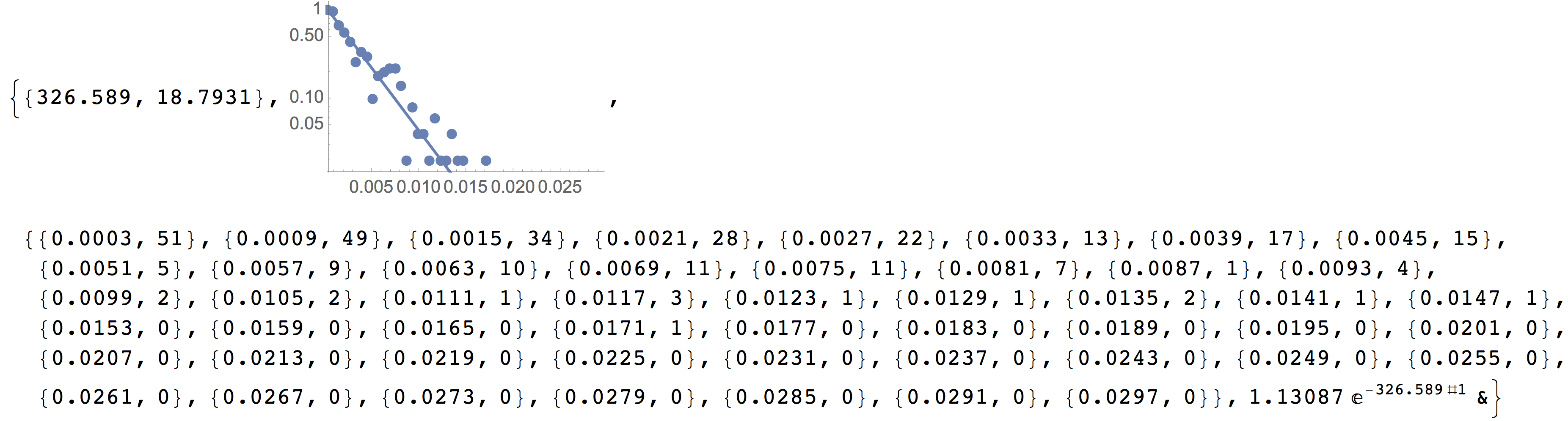
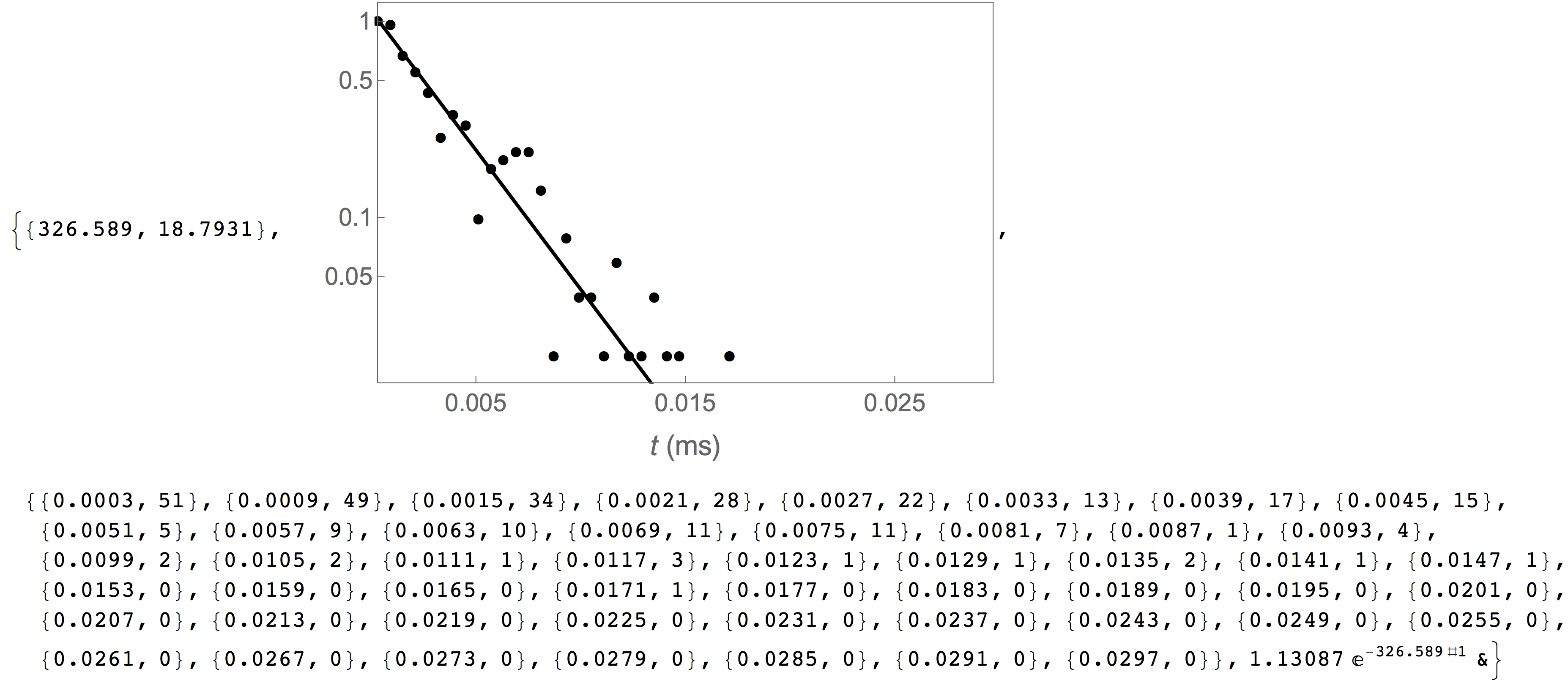
The capture rate plot above can be formatted by supplying the optional plotopts argument, which uses standard Mathematica plot options, as seen in the example below. This is particulary helpful to customize the output of the plot,, for example for publication ready graphics.

       In[4]= CaptureRate[
               QueryDB[
               "<mosaicroot>/data/eventMD-PEG29-Reference.sqlite",
               "select AbsEventStart from metadata where
                       ProcessingStatus='normal' and ResTime > 0.01"
               ], 0.0, 0.05, 50,
               {Frame -> True, FrameLabel -> {Style["t (ms)", 16], ""},
FrameTicks -> {{{0.05, 0.1, 0.5, 1}, None}, {{0.005, 0.015, 0.025},
   None}}, FrameTicksStyle -> 14, PlotStyle -> {Black, Thick},
ImageSize -> 400}
       ]

../_images/mathematica-CaptureRate-Formatted.png

12.2. Matlab¶

The SQLite database output by MOSAIC can be further processed using MATLAB. The data can then be stored in an array in the MATLAB Workspace, and then manipulated as desired.

The features, of opening, querying, and storing as an array, are made available in the MATLAB script openandquery.m. The script does not use the MATLAB Database Manager GUI, a part of the Database Toolbox, which requires a paid license. Instead, an open-source alternative, mksqlite, an interface between MATLAB and SQLite is used.

This section of the manual provides information on how to set up the mksqlite- package for use with MATLAB, and how to use the openandquery.m script.

All code has been successfully tested with MATLAB 2013a, MATLAB 2014a, G++ 4.7 in Ubuntu 14.04 LTS, and Windows Visual C++ 2010. Also, SQLite must be installed prior to performing the following steps.

12.2.1. mksqlite Documentation¶

Information about mksqlite, such as function calls and examples, is available in the MKSQLITE: A MATLAB Interface to SQLite documentation.

12.2.2. Installing mksqlite in Ubuntu 14.04 LTS¶

Download the latest mksqlite source files from SourceForge Unzip the files to a folder, and note the path to that folder (e.g., /home/mksqlitefolder) Open MATLAB, and change the current path to that of the mksqlite folder In the Command Window, type buildit, and press Enter to build mksqlite (this will run the buildit.m script). If the MEX files do not build, one of the following two problems may be why: i) a compiler may not be installed – see the MathWorks page on Supported and Compatible Compilers to select and install a compiler, or ii) errors are generated during compilation of mksqlite.cpp. In the latter case, see the “How to build mksqlite MEX file mksqlite.mexa64 in Linux?” thread in the MathWorks MATLAB Answers forum. If the build proceeds without errors, you will first see the notification “compiling release version of mksqlite…” in the Command Window, followed by “completed.”

Note

GCC/G++ Version (in Linux)

You may have to install a version of GCC/G++ that is compatible with with your specific MATLAB release. If so, check out the linked discussion thread on MATLAB Central on how to set up a MEX Compiler.

12.2.3. Installing mksqlite in Windows 7¶

The installation steps are essentially the same as for Ubuntu, except a different compiler (e.g, contained in Windows SDK 7) may instead have to be installed. If the SDK installer say it cannot proceed, quit the installation, uninstall previous instances of Microsoft Visual C++ 2010, and then install Windows SDK 7 again.

12.2.4. Opening, Querying, and Closing the MOSAIC Output Database¶

The MATLAB script openandquery.m contains all of the commands to: Open a MOSAIC database (e.g., eventMD-PEG29-Reference.sqlite) Query the database Save queried data elements into a structure Close the database Convert the structure into a multi-dimensional array, that can be easily manipulated in MATLAB

Two changes must be made to the openandquery m-file by the end-user: The path to the database file must be changed for each database you wish to access. An example path in Linux would be /home/Data/eventMD-PEG29-Reference.sqlite, and in Windows C:\Data\eventMD-PEG29-Reference.sqlite. The query string can be changed as needed. More information about queries in available in the Database Structure and Query Syntax section.

12.2.5. Example¶

The reference database file provided with MOSAIC is eventMD-PEG29-Reference.sqlite, located in the data folder of the source code root directory. This database contains the results of an analysis performed using the adept2State and consists of the data fields:

{recIDX, ProcessingStatus, OpenChCurrent, BlockedCurrent, EventStart, EventEnd, BlockDepth, ResTime, RCConstant, AbsEventStart, ReducedChiSquared, and TimeSeries}

In the openandquery script modify line 20 by typing in, within the quotes, the correct path to the database file.

dbname = '/home/Data/eventMD-PEG29-Reference.sqlite';

The query in line 23 is to read the names of all fields in the database. The names, along with column ID, and data type, are stored in the structure fieldnames. You may double-click on the variable fieldnames in the Workspace, which will open the structure for you to read the field names in which you are interested.

fieldnames = mksqlite('PRAGMA table_info(metadata)');

Next, modify line 24 to include the query. In this example we want to select (and later manipulate) the data stored in the fields AbsEventStart and BlockDepth. This is where mksqlite comes in: the query are arguments to the mksqlite() function. For more information about using the mksqlite.m function check out the mksqlite documentation.

querytemp = mksqlite('select AbsEventStart, BlockDepth from metadata');

No other changes are required. Run the script. The queried data are stored in the variable data, seen in the MATLAB Workspace (with value 418x2 double). This variable is a 2-column matrix. The first column contains all 418 data elements of the field AbsEventStart, and the second column contains all elements of the field BlockDepth. Note that the query above can be replaced with any standard SQL query as outlined in the Work with SQLite section.

12.3. IGOR¶

Data extraction in IGOR is a work in progress, but a number of users have found a successful route to querying the data and manipulating it in the IGOR environment. The installation and setup for these features requires an understanding of setup and use of ODBC drivers as well as rudimentary programming within the IGOR environment. To date, this has been tested on Mac OS X 10.9. Details may vary for other systems.

12.3.1. Activating SQL Database Access in IGOR¶

Database functionality in IGOR is preloaded, but not activated for use in the standard installation of SQL.xop. To activate this feature follow the instructions detailed in the “Igor Pro Folder/More Extensions/utilities/SQL Help.ihf”. The next few steps are reproduced from the IGOR instructions. First, activate the step in the activation process is open the folder, “Igor Pro Folder/More Extensions/utilities” and create an alias for SQL.xop. Then move the alias to “Igor Pro/Igor Extensions” or a similar folder that is in the search path for IGOR. It may be necessary to delete the “alias” text from the file name for functionality. Restart IGOR to activate.

IGOR relies on an external ODBC driver for database access. Depending on the operating system, it may be necessary to install a stand alone ODBC driver administrator package. First check your machine for the ODBC administrator.app in the ~/Applications/Utilities folder. If not present ODBC administrator can be downloaded directly from the Apple support pages. To test the functionality, it is useful to follow the Installing MySQL ODBC Driver… instructions on the IGOR help page. The MySQL drivers are not necessary for functionally within MOSAIC.

With the ODBC administrator program installed, the next step is to install the SQLite driver for IGOR necessary to interface with the database. Once downloaded run the installation package in “sqlite3-odbc-0.93.dmg” and follow the setup instructions within the disk image. The driver should be ready to use within IGOR.

Hint

The IGOR addon installation (described above) can be activated automatically on Mac OS X by issuing the command python setup.py mosaic_addons --igor from the MOSAIC root directory. Note that administrator privileges are required.

12.3.2. Simple Database Query in IGOR¶

IGOR operates on databases with a single High Level operation command. This one command handles the database connection, query, export of data and closing of the database in one simple function or macro. To access this functionality, first open the procedure window and create the following function:

#include <SQLUtils>

Function QuerySQLData()

        String connectionStr= "DRIVER={SQLite3 Driver};DATABASE='database path';"
        String statement = "select Blockdepth, ResTime from metadata where ProcessingStatus ='normal'"

        SQLHighLevelOp/CSTR={connectionStr, SQL_Driver_COMPLETE}/O/E=1 statement
End

Running this function will extract all normal events and create two waves containing the Blockade depth and Residence time of the events in sequence for further processing in IGOR. Two IGOR functions are included in the /addon/IGOR/ folder that import the data into IGOR waves for further processing. To open these functions to run, simply double click the file and the procedures will be opened in a new IGOR project. Once open, the procedure file can be compiled within IGOR to enable the code. A new menu “Mosaic” should then appear in the title bar within IGOR. A function “Fetch SQL data” will bring up a dialog box to manually enter a search string. After entering the string and clicking continue, you will be prompted to locate the database file you wish to access. The data will be imported into waves with the name automatically imported from the database. Warning: this will overwrite any existing data that is called by identical wave names.