11. Advanced Analysis

We provide packaged functions for advanced analysis such as calculating the capture rate of molecules, determining the residene time, etc as described below.

11.1. Capture Rate

Estimate the capture rate of molecules partitioning into a nanopore.

:Created:    12/27/2015
:Author:     Arvind Balijepalli <arvind.balijepalli@nist.gov>
:License:    See LICENSE.TXT
:ChangeLog:
    12/27/15        AB    Initial version

import numpy as np

from mosaicscripts.analysis.kinetics import CaptureRate

11.1.1. Wrapper Function to Estimate the Capture Rate

The capture rate can be estimated directly by calling the CaptureRate function in mosaicscripts.analysis.kinetics. The function returns a list with two elements: the capture rate (s:math:^{-1}), and the standard error of the capture rate (s:math:^{-1}).

np.round(
        CaptureRate(
            "../data/eventMD-P28-bin.sqlite",
            "select AbsEventStart from metadata where ProcessingStatus='normal' and ResTime > 0.02 order by AbsEventStart ASC"
           ),
        decimals=1
    )

array([ 27.9,   0.2])

11.1.2. Capture Rate Details

from scipy.optimize import curve_fit
import matplotlib.pyplot as plt

from mosaicscripts.analysis.kinetics import query1Col
import mosaicscripts.plots.mplformat as mplformat
from mosaic.utilities.fit_funcs import singleExponential

mplformat.update_rcParams()

Continue reading to dig deeper into how the capture rate is estimated within the CaptureRate function.

The first step is to read in the start times for each event. This is easily done with a query to the MOSAIC database as shown below. The start times are stored in the AbsEventStart column. We limit the events we use to estimate the capture rate to ones that were successfully fit (ProcessingStatus=’normal’) and those whose residence times (ResTime) in the pore are longer than 20 \(\mu\)s.

Finally, we sort the AbsEventStart to ensure the event start times are in ascending order.

start_times=query1Col(
        "../data/eventMD-P28-bin.sqlite",
        "select AbsEventStart from metadata where ProcessingStatus='normal' and ResTime > 0.02 order by AbsEventStart ASC"
    )

Next, we calculate the arrival times, i.e. the time between the start of successive events. This is done with the Numpy diff function. Note that AbsEventStart is stored in milliseconds within the database. Here, we also convert the arrival times to seconds.

arrival_times=np.diff(start_times)/1000.

The partitioning of molecules into the pore is a stochastic process. There are however a couple properties related to stochastic process that we will leverage that makes the estimation of the capture rate more robust. With randomly occuring events that have some mean rate, the number of events scales linearly with time. Therefore, the distribution of these events follows a single exponential form. We can easily test this by calculating the probability density function (PDF) using the Numpy histogram function. Note that the density=True argument normalizes the histogram resulting in a PDF.

density,bins=np.histogram(arrival_times, bins=100, density=True)

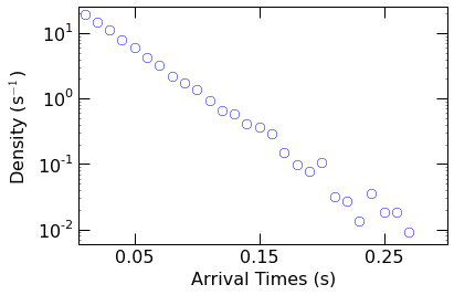
Plot the resulting PDF with Matplotlib to verify the distribution. Sure enough on a semilog scale, the resulting distribution appears linear suggesting an exponential form.

plt.semilogy(
        bins[:len(density)], density,
        linestyle='None',
        marker='o',
        markersize=8,
        markeredgecolor='blue',
        markerfacecolor='None'
    )
plt.xlim(0.005,0.3)
plt.ylim(0.006,25)
plt.xticks([0.05,0.15,0.25])
plt.yticks([1e-2,0.1,1,1e1])
plt.axes().set_xlabel("Arrival Times (s)")
plt.axes().set_ylabel("Density (s$^{-1}$)")
plt.show()

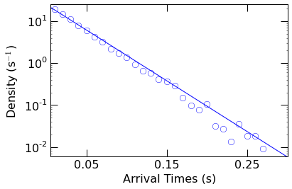
Next we fit the PDF to a single exponential function of the form \(a\ e^{-t/\tau}\), where a is a scaling factor and \(\tau\) is the mean time of the distribution (with a rate of 1/\(\tau\)). This is accomplished with the curve_fit function within Scipy.

popt, pcov = curve_fit(singleExponential, bins[:len(density)], density, p0=[1, np.mean(arrival_times)])

We then visually check the fit, by superimposing the resulting fit function over the PDF.

plt.semilogy(
        bins[:len(density)], density,
        linestyle='None',
        marker='o',
        markersize=8,
        markeredgecolor='blue',
        markerfacecolor='None'
    )
plt.semilogy(
            np.arange(0.001,0.4,0.02),
            singleExponential(np.arange(0.001,0.4,0.02), *popt),
            color='blue'
        )
plt.xlim(0.005,0.3)
plt.ylim(0.006,25)
plt.xticks([0.05,0.15,0.25])
plt.yticks([1e-2,0.1,1,1e1])
plt.axes().set_xlabel("Arrival Times (s)")
plt.axes().set_ylabel("Density (s$^{-1}$)")
plt.show()

Finally, we can extract the capture rate (1/\(\tau\)) from the optimal fit parameters.

np.round([1/popt[1]], decimals=1 )

array([ 27.9])