4. MOSAIC GUI
MOSAIC’s GUI interface is designed to allow you to easily setup and run an analysis and to analyze the results of prior trials via a graphical interface; it contains the most commonly used features of MOSAIC. The GUI contains modular panels for setting up an analysis, running it, and analyzing the results. Here we give you a brief overview of the graphical interface and its basic use. You can learn more in the Examples section.
Opening the GUI
If you installed MOSAIC from a precomiled binary, you can open the GUI by double clicking the MOSAIC icon. Alternatively, if you compiled MOSAIC from source code, you can run the GUI from the terminal window – navigate to the installation directory and type:
python runMOSAIC
Hint
Having trobule getting the GUI to start? Frequently, this arises because your PYTHONPATH environment variable is set up incorrectly. To fix this error, first type echo $PYTHONPATH in the terminal. If you don’t see the path to the MOSAIC installation in PYTHONPATH, consult the operating-system specific instructions (OSX or Ubuntu) to help resolve this issue.
4.1. Interface Overview
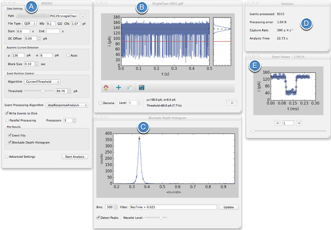
Primary panels in MOSAIC: (A)Analysis Setup (B) Trajectory Viewer (C) Live Blockade Depth Histogram (D) Live Analysis Statistics (E) Event Viewer.
The main interface consists of five panels which we go over in detail later in this document. Briefly, these are:
Analysis Setup: This panel is used to set up the analysis parameters.
Trajectory Viewer: This panel shows a snippet of the ionic current time-series and an all points histogram, used to set the baseline and threshold parameters found in Panel A: Analysis Setup.
Blockade Depth Histogram: Once the data processing has started, this panel shows a live blockade depth histogram; a query can be defined to restrict the histogram to data which fulfills a user-defined criteria.
Analysis Statistics: Displays live statistics about the data processed.
Event Viewer: Displays the partitioned events and their fit. This panel is active only if “Write Events to Disk” is enabled in the Analysis Setup.
4.2. Panels A & B: Analysis Setup and Trajectory Viewer
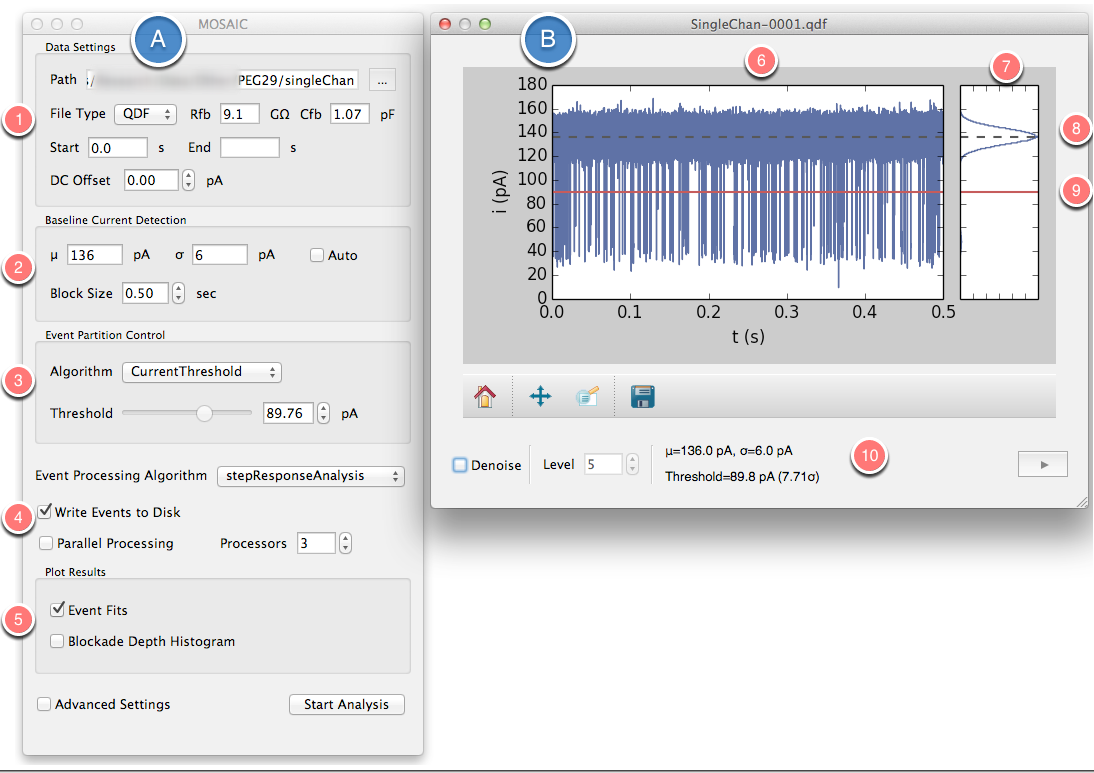
Overview of Panels A & B: (A) Analysis setup panel (B) Trajectory viewer panel
4.2.1. Panel A: Analysis Setup
1. Data Settings
Path: Allows user to set the directory containing files to analyze. Click the “…” icon to navigate to the directory.
File Type: The GUI is natively compatible with either ABF or QDF Files, this field is automatically populated based on the files in the directory you’ve chosen.The Rfb and Cfb parameters are needed to correctly analyze QDF files (see
qdfTrajIOfor more information)Rfb & Cfb: MOSAIC supports the QUB QDF file format used by the Electronic Biosciences Nanopatch system. Two additional parameters, the feedback resistance (Rfb) in Ohms and capacitance (Cfb) in Farads are required to appropriately convert the measurements to ionic current.
Start and End: These parameters allow you to analyze a range of your data. Choose the starting and ending times if you’d like to analyze a small time segement of your data. If this is left blank, all data will be analyzed.
DC Offset: If your measurement contains a systematic bias, it can be manually corrected by entering the DC offset here.
2. Baseline Current Detection
\(\mu\): Mean baseline current, in picoamperes (pA). This is shown schematically in the trajectory viewer (see Label #8). When Auto is selected, this will be greyed out and labeled
<auto>\(\sigma\): Noise level (in pA). This is expected noise level of your baseline. Typically one would set this to the measured RMS noise of the open channel state at the cutoff frequency. When Auto is selected, this will be greyed out and labeled
<auto>.Auto: Checking this box enables automatic dectection of the mean baseline current (\(\mu\)) and noise level (\(\sigma\)). When auto is enabled, the values chosen by the software will be displayed in the trajectory viewer panel (see Label #10)
Block Size: Controls the amount of data examined to determine the baseline. This also controls the amount of data shown in the trajectory viewer.
3. Event Partition Control
This panel is used to set the current threhold used for event detection
Algorithm: Currently,the only event partitioning algorithm enabled is CurrentThreshold.
Threshold: This is used to set the minimum current threshold used to partition events with the CurrentThreshold algorithm.
4. Event Processing Setup
Event Processing Algorithm: The GUI supports two event processing algorithms, i) StepResponseAnalysis and ii) MultiStateAnalysis. StepResponseAnalysis is the default analysis, and should be used with data sets with unimodal events. For events with mutliple states or steps the MultiStateAnalysis algorithm, which is capable of automatically analyzing events with N states, should be used. Note that StepResponseAnalysis is a restricted case of MultiStateAnalysis and is more computationally efficient to run if you have unimodal (or single states) data.
Write Events to Disk: When this box is checked, the data points for each partition events are written to the SQLite database. When this is checked it is possible to view the individual fits of each in the Event Fits panel.
Hint
When Write Evens to Disk is checked, your database can become extremely large! This is because MOSAIC is effectively writing most of your time-series to the database. Note that the fit parameters are always written to the database.
Parallel Processing and Processors: Parallel processing can be enabled by checking this box. This box will be greyed out if the python module ZeroMQ is not installed. The Processors box allows you to select the number of processors used in the analysis. It is important to note that the GUI will occupy one processor, so choosing 3 processors will actually use a total of 4 processors.
5. Plot Results and Advanced Settings
Event Fits: Checking this box will show the events viewer (Panel E). This can also be accessed from the file menu
View>Plots>Event Fits. If Write Events to Disk is not enabled this checkbox will be greyed out.Blockade Depth Histogram: Checking this box will show the blockade depth histogram (Panel C). This can also be accessed through the file menu
View>Plots>Blockade Depth Histogram.Advanced Settings: This opens a dialog window to manually edit settings not otherwise accessible in the GUI. See the Settings File section for further details.
4.2.2. Panel B: Trajectory Viewer
This panel shows a segment of the data time series. The file currently being displayed is shown at the top of the window. If data from multiple files are loaded, the last filename is displayed. The length of time displayed in the window is controlled by BlockSize in Panel A (see #2).
6. Time Series (Trajectory)
This plot shows the ionic current time series, of length BlockSize. Other features in the panel (such as histogram, denoising, etc.) only utilize the data in the window for their calculations.
7. All Points Histogram
This shows a histogram of the time series data shown in #6.
8. Dashed line indicates mean baseline current
9. Detection threshold level indicated by solid red line
10. Navigation, Denoising, and Statistics
Navigation Tools: Tools to navigate the plot window are shown below the time-series plot. These can be applied to either the trajectory or all points histogram plots. The arrow bar on the bottom right of the trajectory viewer can be used to advance to the next data block.
Denoising Wavelet denoising can be activated by clicking , the denoising level is enabled here, the level of denoising can be varied between 1 and 5.
Warning
Wavelet-based denoising is currently an experimental feature and should be used with caution.
Baseline Statistics: The mean baseline current, standard deviation, and the threshold used for event detection (specified as a multiple of the standard deviation in parenthesis) correspond to the settings in the main window. If the baseline current detection is set to auto these values will update as each data segment is examined. The size of this segment is determined by the Block Size setting. In the figure above, the Block Size is set to 0.5 s.
4.3. Panels C,D, & E: Blockade Depth Histogram, Statistics, and Event Viewer
4.3.1. Panel C: Blockade Depth Histogram
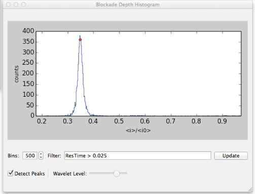
Blockade depth histogram
This window shows the blockade depth histogram calculated from the meta-data output by MOSAIC.
Filter: The data displayed in the histogram can be restricted to events that fulfill specific user-defined criteria. For instance, the default filter
ResTime > 0.025only includes events longer than 0.025 ms (or 25 \(\mu s\)). The GUI uses a SQL select statement to restrict the events included in the histogram. The text in the Filter field represents the part of the query after the where clause, and allows the user to use standard SQL syntax to narrow the results in the plot. See the Work with SQLite section for details on SQL syntax.Bins: The number of bins in the histogram are defined here. By default, 500 bins are used, but the user can change this necessary.
Detect Peaks: Checking Detect Peaks enables a wavelet-based peak detection algorithm. The wavelet level slider controls the sensitivity of the peak detection. Sliding it to the right will decrease the number of peaks picked up. The peaks detected are represented with red dots. Mousing over the detected peaks cause the coordinates of the peak to be displayed in the lower right hand corner of the window. The detected peaks can also be exported to a CSV file from the file menu
File>Save Histogram.
4.3.2. Panel D: Statistics
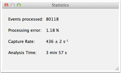
Live statistics window
The Statistics Window is displayed when a new analysis is started and displays:
Events Processed: The number of events processed.
Processing Error: The processing error rate (i.e. the percentage of events for which fit has failed).
Capture Rate: An estimate of the mean capture rate.
Analysis Time: The amount of data processed (in seconds).
4.3.3. Panel E: Event Viewer
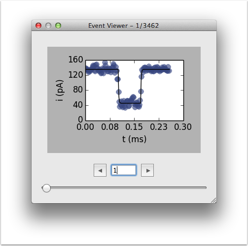
Event viewer window
If Write to Disk is enabled, this panel allows you to view the first 10,000 events processed. This is useful to ensure the quality of the analysis and to debug potential problems with the settings.
4.3.4. Console Log
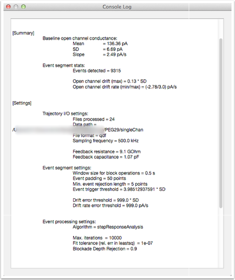
Console log window
When processing is complete, this panel displays a log of the analysis. This log contains useful information such as the analysis settings, the number of events fit, baseline drift, open channel conducatance, etc. This file is written to the database and can be accessed later.
4.3.5. Advanced Settings
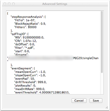
Advanced settings window
This dialog allows you to manually edit advanced settings for uncommon use cases not natively accessible from within the GUI. Further information can be found in the Settings File.