Mathematica
Installation
The analysis output generated by MOSAIC can be imported into Mathematica for further processing. This accomplished with two packages: the low level MosaicUtils and MosaicAnalysis, which contains additional analysis routines. The addon package must first be installed to one of the locations in the Mathematica path. Alternatively, the required package files can be installed to the Applications folder using setuptools on Mac OS X and Linux by issuing the command below in the root folder of the MOSAIC code. Instructions for installing the package files for Windows are available here.
python setup.py mosaic_addons --mathematica
MosaicUtils
MosaicUtils provides low level functions to interact with a database output by MOSAIC. MosaicUtils can use a native Mathematica (slower, default) or Python (faster, but experimental) backend to query databases output by MOSAIC.
Note
To select the Python backend, please call the SetQueryBackend function as described below. If you use a virtual environment with Python, please call the SetVirtualEnv function after you install this addon.
SetQueryBackend[backend]
- Args:
backend : select the Mathematica (default) or Python (faster, experimental) backend to run SQLite queries.
- Returns:
None
ReadQueryBackend[]
- Args:
None
- Returns:
The backend used to run SQLite queries.
SetVirtualEnv[virtualenv]
- Args:
virtualenv : name of the virtual environment configured for use with MOSAIC
- Returns:
None
PrintMDKeys[dbfile]
Returns a list of column headings from the metadata table.
- Args:
dbfile : full path to the database file
- Returns:
A list of column names in the table metadata.
PrintMDTypes[dbfile]
Returns a list of column types from the metadata table.
- Args:
dbfile : full path to the database file
- Returns:
A list of column types in the table metadata.
QueryDB[dbfile, query]
Queries the metadata table using the supplied SQL query.
- Args:
dbfile : full path to the database file
query : a SQL query
- Returns:
A nested list of query results.
PlotEvents[dbfile, FsKHz, nEvents]
Plot the event-time series if stored in the database (see the Settings File section for details on saving time-series to the analysis output).
- Args:
dbfile : full path to the database file
FsKHz : sampling frequency in kHz.
nEvents : (optional) limit the plot to the first
nentries in the database
- Returns:
A dynamic object that allows the user to browse event time-series and fits.
GetAnalysisAlgorithm[db]
Returns the analysis algorithm used to process the current data set.
- Args:
db : full path to a database file
- Returns:
Algorithm used to analyze data.
MosaicUtils Examples
Once installed as described above, MosaicUtils must be imported as shown below.
In[1]= <<MosaicUtils`
SQL queries require the exact column names when querying data from a table (see Database Structure and Query Syntax). Column names in the metadata table, which stores the main results from the analaysis can be retrieved using the PrintMDKeys function as shown below. In this example, the column names returned correspond to an analysis performed using the adept2State algorithm.
In[2]= PrintMDKeys["<mosaicroot>/data/eventMD-PEG29-Reference.sqlite"]

Out[2]= {"recIDX", "ProcessingStatus", "OpenChCurrent",
        "BlockedCurrent", "EventStart", "EventEnd",
        "BlockDepth", "ResTime", "RCConstant", "AbsEventStart",
        "ReducedChiSquared", "TimeSeries"
        }
The MosaicUtils package allows the output of MOSAIC to be queried just like from Python. This accomplished using the QueryDB function. In the example below, we retrieve a column that returns the start time of the first 10 entries in the metadata table that have their ProcessingStatus set to normal. The results are then returned in a standard list. Note that QueryDB accepts a standard SQL query as described in more detail in the Database Structure and Query Syntax section.
In[3]= QueryDB[
        "<mosaicroot>/data/eventMD-PEG29-Reference.sqlite",
        "select AbsEventStart from metadata where ProcessingStatus='normal' limit 10"
        ]

Out[3]= {
        {1.84376}, {4.54439}, {5.26933}, {6.01253}, {6.80369},
        {8.48988}, {10.841}, {11.2246}, {13.2892}, {16.3983}
        }
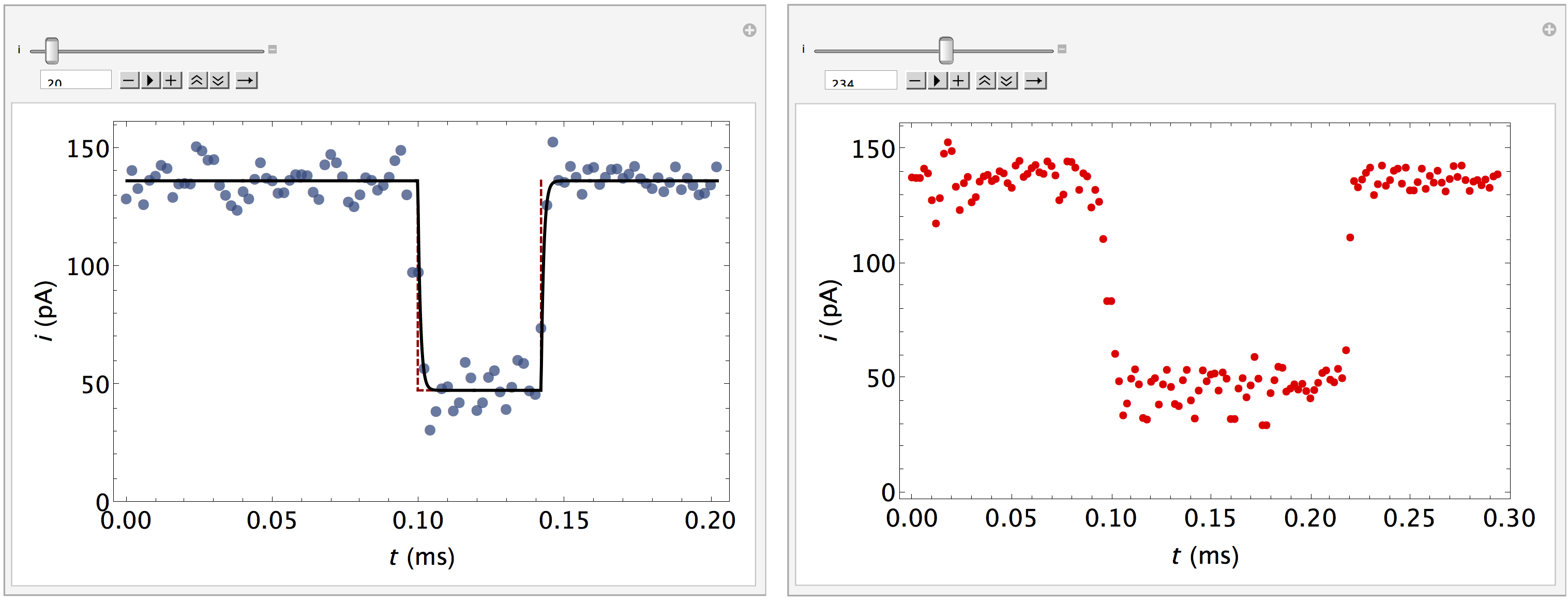
Finally, the addon package allows us to plot individual events if time-series data was stored in the database. This is accomplished using the PlotEvents function, and provides a convenient tool to visually inspect the output of a MOSAIC analysis. In the example below, we inspect the events stored in the reference PEG28 data set included with MOSAIC. PlotEvents returns a dynamic object that allows the user to inspect all the events in a database. An event that was properly characterized by the code is plotted with blue markers (left). The plot is overlaid with the optimized fit function (black) and an idealized pulse (red dashed). Events that were not properly fit are plotted with red markers (right).
In[4]= PlotEvents["<mosaicroot>/data/eventMD-PEG29-Reference.sqlite", 500]
MosaicAnalysis
MosaicAnalysis builds on the MosaicUtils package and provides basic analysis functions such as estimating the capture rate of molecules partitioning into a channel, or the mean residence time. Additionally, new functionality can be created by combining the functions defined below.
ScaledSingleExponentialFit[hist, lambda, lambda0]
Scale the histogram with the number of counts in the first bin. Fit a single exponential of the form a exp(-t/tau) to the scaled histogram.
- Args:
hist : a histogram with format {{bin1, counts1}, {bin2, counts2}, …, {binN,countsN}}
lambda : parameter of the distribution. This symbol must be passed from the calling function.
lambda0 : initial guess for lambda.
PlotScaledSingleExponentialFit[hist, ftfunc, plotopts]
- Args:
hist : a histogram with format {{bin1, counts1}, {bin2, counts2}, …, {binN,countsN}}
ftfunc : an optimized fit, defined as a virtual function.
plotopts: a list of options to control the plot output.
CaptureRate[arrtimes, stime, etime, nbins, plotopts]
Estimate the capture rate of molecules by a channel by analyzing the arrival times of individual molecules. The arrival times of a stochastic process follow a single exponential distribution. This function first calculate a histogram of arrival times and then fits a single exponential function to the data.
- Args:
arrtimes : a list of absolute start times (AbsEventStart) queried from a database.
stime : lower limit of the arrival times distribution
etime : upper limit of the arrival times distribution
nbins : number of bins
plotopts : a list of options to control the plot output.
- Returns:
The mean capture rate, a plot of the underlying distribution of arrival times, the arrival times distribution and the optimized fit function.
ArrivalTimes[abseventstart]
Calculate the arrival times from a list of the absolute start time of each event in a data set.
- Args:
abseventstart : a list of absolute start times (AbsEventStart) queried from a database.
- Returns:
A list of arrival times.
MosaicAnalysis Examples
In[1]= <<MosaicUtils`
In[2]= <<MosaicAnalysis`
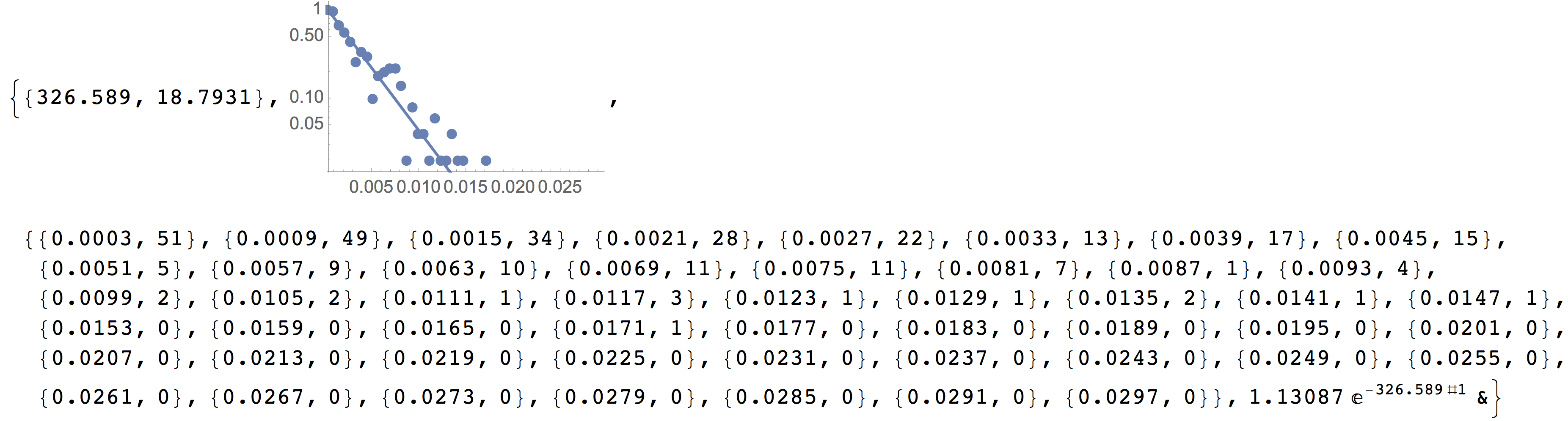
In the following example, we estimate the capture rate of PEG28 from the reference data set included with the MOSAIC source. The first argument fo CaptureRate is a list of the absolute start time of each event in the database. This data can be obtained using the query shown below. The remaining arguments to CaptureRate define the parameters of the arrival times distribution, the lower and upper limit of the arrival times and the number of bins. The function returns the mean capture rate and standard error, a plot that shows the underlying arrival times distribution, raw data used to generate the capture rate histogram, and a pure best-fit function.
In[3]= CaptureRate[
        QueryDB[
        "<mosaicroot>/data/eventMD-PEG29-Reference.sqlite",
        "select AbsEventStart from metadata where
                ProcessingStatus='normal' and ResTime > 0.01"
        ], 0.0, 0.05, 50
]
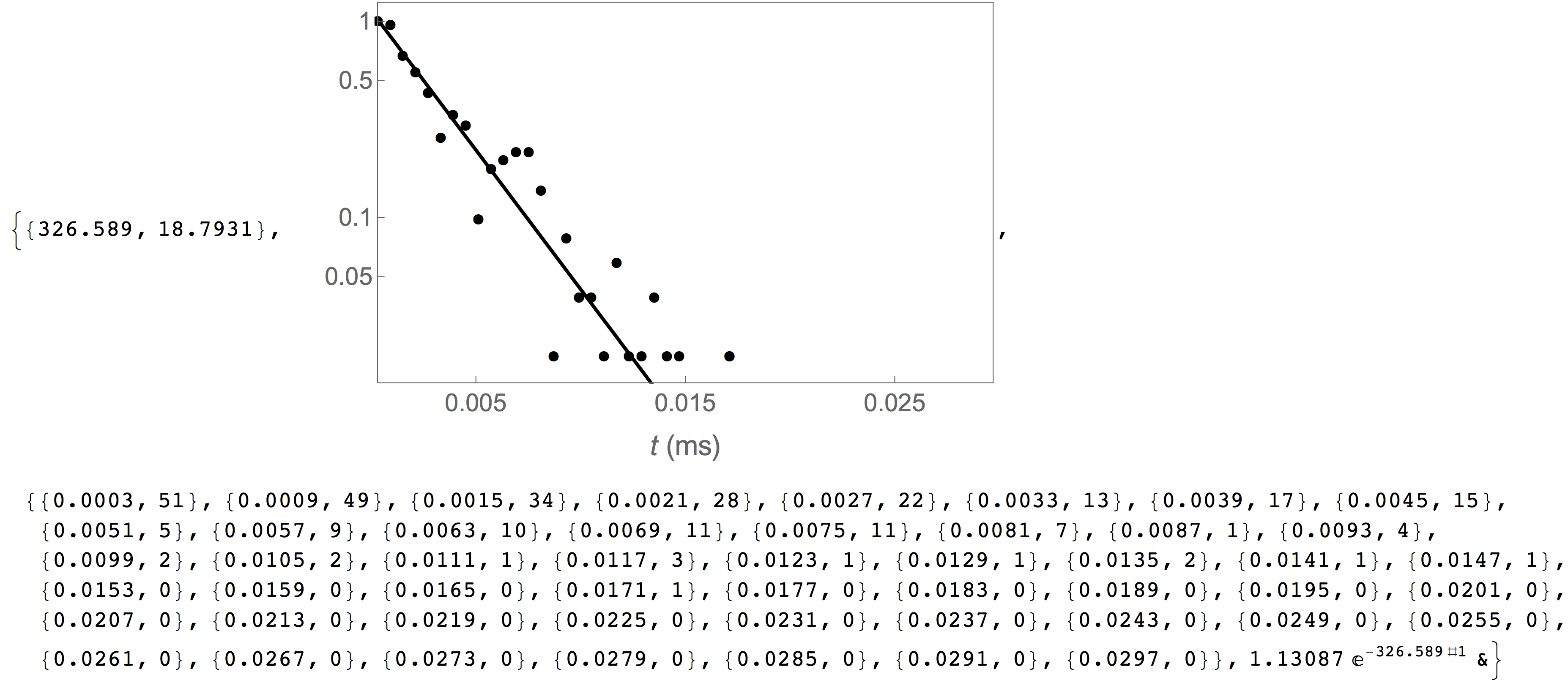
The capture rate plot above can be formatted by supplying the optional plotopts argument, which uses standard Mathematica plot options, as seen in the example below. This is particulary helpful to customize the output of the plot,, for example for publication ready graphics.
       In[4]= CaptureRate[
               QueryDB[
               "<mosaicroot>/data/eventMD-PEG29-Reference.sqlite",
               "select AbsEventStart from metadata where
                       ProcessingStatus='normal' and ResTime > 0.01"
               ], 0.0, 0.05, 50,
               {Frame -> True, FrameLabel -> {Style["t (ms)", 16], ""},
FrameTicks -> {{{0.05, 0.1, 0.5, 1}, None}, {{0.005, 0.015, 0.025},
   None}}, FrameTicksStyle -> 14, PlotStyle -> {Black, Thick},
ImageSize -> 400}
       ]