Model system: 1D ideal gas in a linear external potential

Below we gain intuition for the analytical model included in the thermoextrap package. Specifically, we have a system with \(N\) ideal gas (IG) particles with a single dimension of length \(L\). The potential energy for each particle is only a function of the particle location, \(U(x) = ax\) where \(x\) is the position of a particle along the single dimension. In what follows, \(\beta=\frac{1}{k_{B}T}\) is the inverse temperature and we set the energy associated with particular position due to the external potential, \(a\), equal to 1. This does not lose any generality as only values of \(\beta\) or \(L\) relative to \(a\) matter.

Though this system is simple and completely analytical, it can be used to test nearly all of the functionalities of the thermoextrap package. As a result, it is featured in the unit testing to ensure that the code is not only reproducible, but also produces physically correct results coinciding with theory. This code is located in the module thermoextrap.idealgas.

%matplotlib inline

import cmomy
import matplotlib.pyplot as plt
import numpy as np

from thermoextrap import idealgas

rng = cmomy.random.default_rng(seed=0)

beta = 1.0
npart = 1000
nconfig = 10000

fig, axes = plt.subplots(3, 2)


def get_utest(npart, beta, vol, ndev=5, n=100):
    uave = idealgas.x_ave(beta, vol) * npart
    ustd = np.sqrt(idealgas.x_var(beta, vol) * npart)
    return np.linspace(-1.0, 1.0, n) * ndev * ustd + uave


# Note for ideal gas model, vol = length
vols = [1.0, 10.0]

for vol, ax in zip(vols, axes.T):
    xvals = np.arange(0.0, vol, 0.0001)

    # There are functions to sample both position and potential energy values
    uvals = idealgas.u_sample((nconfig, npart), beta, vol)
    uhist, ubins = np.histogram(uvals, bins="auto", density=True)
    ubincents = 0.5 * (ubins[:-1] + ubins[1:])

    # We can also just directly calculate the average or variance of the particle positions
    utest = get_utest(npart, beta, vol)

    # Or you can get the probability distribution of x or U
    ax[0].set_title(f"L={vol}")
    ax[0].plot(xvals, idealgas.x_prob(xvals, beta, vol))
    ax[1].plot(xvals, idealgas.x_cdf(xvals, beta, vol))
    ax[2].plot(ubincents, uhist, "o")
    ax[2].plot(utest, idealgas.u_prob(utest, npart, beta, vol))

for a in axes[1, :]:
    a.set_xlabel("x")
for a in axes[2, :]:
    a.set_xlabel(f"U for N={npart}")
for a, label in zip(axes[:, 0], ["P(x)", "cdf(x)", "P(U)"]):
    a.set_ylabel(label)

fig.tight_layout()

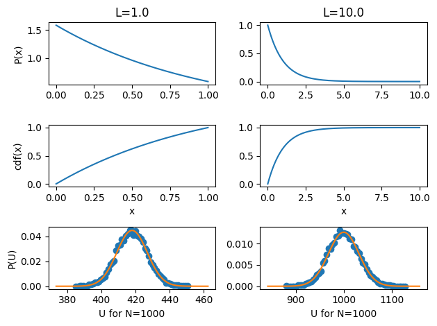
The probability of a particle residing at a particular location is \(\frac{e^{-\beta a x}}{\int_0^L e^{-\beta a x} dx}\), shown in the top panel. The cumulative distribution function, which is used to randomly sample from the distribution \(P(x)\), is shown in the middle. From \(N\) random draws of \(x\) distributed according to \(P(x)\), you have a single configuration with \(N\) particles. The potential energy for a single configuration is \(a \sum_i x_i\) and so by randomly sampling many configurations, we construct the potential energy distribution in the bottom panel. For a single particle, the potential energy distribution is identical to \(P(x)\) since a single \(x\) maps to exactly one potential energy. For many particles, however, the potential energy is a random variable composed of a sum of independent random variables and so the distribution is Gaussian, as confirmed by the bottom panel.

# Now look at behavior as a function of inverse temperature (at the same system sizes as above)

betas = np.arange(0.1, 10.0, 0.5)
colors = plt.cm.coolwarm_r(np.arange(0.0, 1.0, float(1.0 / len(betas))))

fig, axes = plt.subplots(3, 2)

for vol, ax in zip(vols, axes.T):
    xvals = np.arange(0.0, vol, 0.0001)
    ax[0].set_title(f"L={vol}")
    ax[0].plot(betas, idealgas.x_ave(betas, vol))

    for beta, color in zip(betas, colors):
        ax[1].plot(xvals, idealgas.x_prob(xvals, beta, vol), color=color)
        utest = get_utest(npart, beta, vol)
        ax[2].plot(utest, idealgas.u_prob(utest, npart, beta, vol), color=color)

    ax[0].set_xlabel(r"$\beta$")
    ax[0].set_ylabel(r"$\langle x \rangle$")
    ax[1].set_xlabel("x")
    ax[1].set_ylabel("P(x)")
    ax[2].set_xlabel(f"U for N={npart}")
    ax[2].set_ylabel("P(U)")


fig.tight_layout()

plt.show()

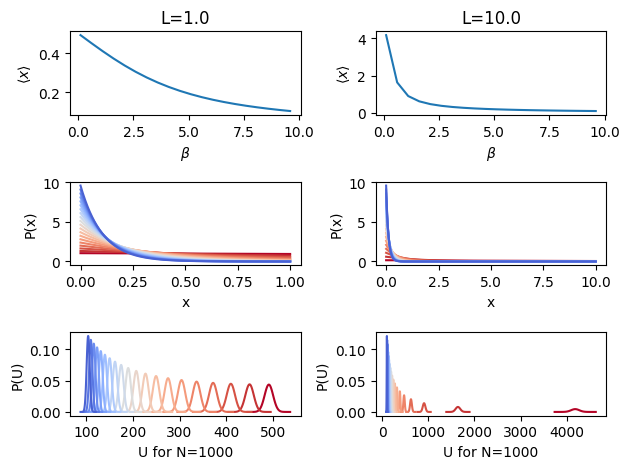
A simple structural property of interest is the average \(x\) value, which is plotted in the top panel as a function of \(\beta\). It’s only non-linear over a very large temperature range, but it’s a toy system so the physical temperature really isn’t relevant anyway. Changes in \(P(x)\) and \(P(U)\) with temperature are shown as well with coloring by temperature, NOT inverse temperature (blue is the lowest \(T\), highest \(\beta\)). Clearly the configurational distributions will not overlap in their important regions and neither will the potential energy distributions, meaning perturbation won’t work at some point. This is especially true as \(L\) is increased.

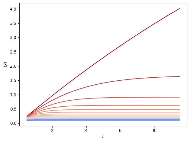
Below, we show \(\langle x \rangle\) as a function of \(L\) at various temperatures. Non-linearities arise at all temperatures to varying degrees.

# Behavior of average x as a function of L
fig, ax = plt.subplots()
vols = np.arange(0.5, 10.0, 0.5)

for beta, color in zip(betas, colors):
    ax.plot(
        vols,
        idealgas.x_ave(beta, vols),
        color=color,
        label=rf"$\beta$ = {beta}",
    )

ax.set_xlabel(r"$L$")
ax.set_ylabel(r"$\langle x \rangle$")

fig.tight_layout()

plt.show()

For testing for physical accuracy, note that the thermoextrap.idealgas module also comes with analytical computations of the derivatives with respect to \(\beta\) of \(\langle x \rangle\), \(\langle \beta x \rangle\), \(-\ln \langle x \rangle\), and \(-\ln \langle \beta x \rangle\). This allows for “exact” extrapolations at a given order, or at least what the extrapolation at that order should be in the limit of infinite sampling. There is also a function to compute analytical derivatives, and hence extrapolations, with respect to \(L\). As we will explore in other notebooks, these scenarios cover most cases of interest in extrapolating structural and thermodynamic properties. For more information, see here.