Macrostate distribution extrapolation

This notebook demonstrates how to perform temperature extrapolation (or interpolation) of macrostate log-probability distributions \(\ln \Pi (N)\) for the number of particles from a flat-histogram grand canonical ensemble simulation.

%matplotlib inline

We start by setting up functions to load in the data.

# Need to load in some data, partially specifying information about simulations here
# As well as functions to load data
import glob

import matplotlib.pyplot as plt
import numpy as np
import xarray as xr


def get_sim_activity(Tr) -> float:
    if Tr == 0.700:
        return -6.250
    if Tr in {0.73, 0.74}:
        return -5.500
    if Tr == 0.850:
        return -4.800
    if Tr == 1.100:
        return -3.380
    if Tr == 1.200:
        return -3.000

    raise ValueError("Reduced temperature %f outside range in dataset." % Tr)


def get_file_prefix(Tr, run_num=None):
    base_str = "./SRS_data/lj.t%s.n12m6.v512.rc3.b.r" % (
        str("%1.2f" % Tr).replace(".", "")
    )
    if run_num is not None:
        return ["%s%i" % (base_str, run_num)]
    unstripped = glob.glob("%s*.energy.dat" % base_str)
    return [u[:-11] for u in unstripped]


def load_data(Tr, ref_mu=-4.0, run_num=None):
    f_prefixes = get_file_prefix(Tr, run_num=run_num)
    U_moms = np.array(
        [np.loadtxt("%s.energy.dat" % f)[:, 1:] for f in f_prefixes]
    )  # Reduced units of energy/eps
    lnPis = np.array([np.loadtxt("%s.lnpi.dat" % f)[:, 1] for f in f_prefixes])
    N_vals = np.array([np.loadtxt("%s.lnpi.dat" % f)[:, 0] for f in f_prefixes])
    mu = Tr * get_sim_activity(
        Tr
    )  # Tr is kB*T/eps, activity is mu/kB*T, so getting mu/eps

    # Convert to x_arrays with proper labeling
    # Potential energy data is average U and average U^2 at each bin N for each repeat
    # So dimension are N_repeats by N by 2
    # And don't forget to include 0th order moments (all 1s)
    U_moms = np.concatenate([np.ones_like(lnPis)[..., None], U_moms], axis=-1)
    U_moms = xr.DataArray(U_moms, dims=["rec", "n", "umom"])
    # For lnPi, adjust to a reference mu value
    # And subtract off N=0 bin
    lnPis = lnPis + (
        (1.0 / Tr) * (ref_mu - mu) * N_vals
    )  # Multiply by 1/Tr since want beta*mu
    lnPis = lnPis - lnPis[:, :1]
    lnPis = xr.DataArray(lnPis, dims=["rec", "n"])
    # For mu need to add extra axis called comp
    ref_mu = xr.DataArray(ref_mu * np.ones((len(f_prefixes), 1)), dims=["rec", "comp"])

    return {
        "energy": U_moms,
        "lnPi": lnPis,
        "mu": ref_mu,
        "mu_sim": mu,
        "beta": 1.0 / Tr,
    }

And actually load in the data to use for extrapolation/interpolation. This data is from simulations of in the grand canonical ensemble with flat-histogram methods employed to enhance sampling in the particle number. The potential considered is Lennard-Jones fluid, with more information found here.

temps = np.array([0.70, 0.73, 0.74, 0.85, 1.10, 1.20])
betas = (
    1.0 / temps
)  # Reduced temperature is Tr = kB*T/eps, so beta is also dimensionless as eps/kB*T

data_dicts = [load_data(t) for t in temps]

Extrapolation

We will start out by extrapolating from a central temperature value, moving both higher and lower.

We need to import thermoextrap generally for access to data classes, then lnpi for special functions related to derivatives of macrostate distributions.

import thermoextrap as xtrap

First, we need to create a data object to hold the data. Selecting the data, however, requires a bit of thought. Though we are interested in extrapolating \(\ln \Pi (N)\), it turns out it is more convenient (and equivalent within an additive constant) to extrapolate \(\ln \Pi (N) - \ln \Pi (0)\). The first two derivatives of this with respect to \(\beta = \frac{1}{k_B T}\) are:

    \(\frac{\mathrm{d} \ln ( \Pi (N)/\Pi(0) )}{\mathrm{d} \beta} = \mu N - \langle U \rangle_N\)
    \(\frac{\mathrm{d}^2 \ln ( \Pi (N)/\Pi(0) )}{\mathrm{d} \beta^2} = - \frac{\mathrm{d} \langle U \rangle_N}{\mathrm{d} \beta}\)

The chemical potential is given by \(\mu\) and the angle brackets with a subscript of \(N\) represent a canonical ensemble average at a particular macrostate with \(N\) particles. While the first derivative involves \(\mu N\) and the potential energy, it is clear that for \(k > 1\),

    \(\frac{\mathrm{d}^k \ln ( \Pi (N)/\Pi(0) )}{\mathrm{d} \beta^k} = - \frac{\mathrm{d}^{k-1} \langle U \rangle_N}{\mathrm{d} \beta^{k-1}}\)

What this means is that all we need is a way to compute canonical ensemble derivatives of an average observable with respect to \(\beta\), which we have in thermoextrap.beta, and a custom derivative function to handle the special case of the 0\(^\mathrm{th}\) and 1\(^\mathrm{st}\) derivatives. This has been implemented in thermoextrap.lnpi for convenience.

Based on the discussion above, we start by creating a custom data callback object that helps manage how derivatives are calculated and what information is provided to the function that calculates the derivatives.

# for lnPi extrapolation, we need to setup a DataCallback
# see definition in xtrap.lnpi
ref = data_dicts[3]
meta_lnpi = xtrap.lnpi.lnPiDataCallback(
    ref["lnPi"], ref["mu"], dims_n=["n"], dims_comp="comp"
)

In the above callback, the first argument is the reference \(\ln \Pi\) we’re extrapolating from, the second argument is the chemical potential \(\mu\), dims_n is the dimension of the input DataArray over which the particle number \(N\) changes, and if you really want to understand what dims_comp is you’ll have to ask Bill.

Next we need a data object to hold the potential energy moments, passing the callback as the meta argument. Note that because we’re working with potential energies only, we can set xu=None and x_is_u=True to provide further accelerations for this special case.

data_lnpi = xtrap.DataCentralMoments.from_ave_raw(
    u=ref["energy"], xu=None, x_is_u=True, central=True, meta=meta_lnpi
)

And finally, use that data to create our extrapolation model.

em_lnpi = xtrap.lnpi.factory_extrapmodel_lnPi(beta=ref["beta"], data=data_lnpi, order=1)

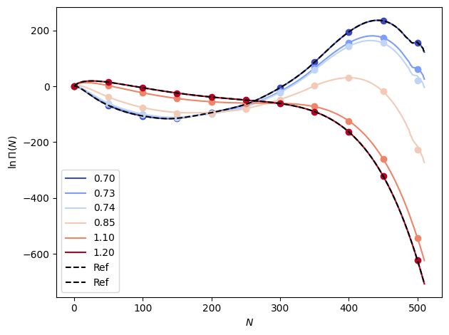
We can make predictions at a range of beta values for which we have data to check (in the loaded “samples” data). Note that we set all \(\ln \Pi (0)\) elements to zero.

out_lnpi = em_lnpi.predict(betas).mean(dim="rec")
out_lnpi -= out_lnpi.sel(n=0)

# Plot the results
fig, ax = plt.subplots()

colors = plt.cm.coolwarm(np.linspace(0.0, 1.0, len(betas)))

n_vals = np.arange(out_lnpi.sizes["n"])

for i, b in enumerate(betas):
    ax.plot(n_vals, out_lnpi.sel(beta=b), color=colors[i], label="%1.2f" % temps[i])
    ax.plot(
        n_vals[::50],
        data_dicts[i]["lnPi"].mean(dim="rec").values[::50],
        "o",
        color=colors[i],
    )

ax.plot(n_vals, ref["lnPi"].mean(dim="rec"), "k--", label="Ref")

ax.set_xlabel(r"$N$")
ax.set_ylabel("$\\ln \\Pi (N)$")

ax.legend()

fig.tight_layout()

plt.show()

This extrapolation misses too far away from the reference. Next we will try interpolation using up to first-order derivatives, which gives us a 3rd order interpolating polynomial.

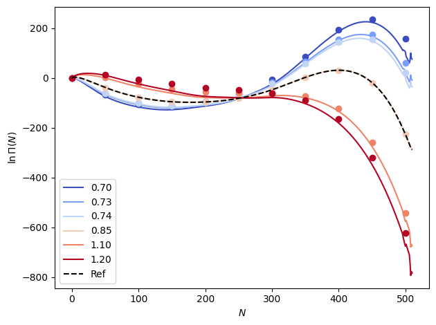
Interpolation

Implementing interpolation is easy if we already have thermoextrap.models.ExtrapModel objects. So just need to build a list of these for the end states (highest and lowest temperatures) we will use as our references.

xems_interp = []
for d in [data_dicts[0], data_dicts[-1]]:
    this_meta = xtrap.lnpi.lnPiDataCallback(
        d["lnPi"], d["mu"], dims_n=["n"], dims_comp="comp"
    )
    this_data = xtrap.DataCentralMoments.from_ave_raw(
        u=d["energy"], xu=None, x_is_u=True, central=True, meta=this_meta
    )
    this_xem = xtrap.lnpi.factory_extrapmodel_lnPi(
        beta=d["beta"], data=this_data, order=1
    )
    xems_interp.append(this_xem)

xemi = xtrap.InterpModel(xems_interp)

out_xemi = xemi.predict(betas).mean(dim="rec")
out_xemi -= out_xemi.sel(n=0)

# Plot the results
fig, ax = plt.subplots()

colors = plt.cm.coolwarm(np.linspace(0.0, 1.0, len(betas)))

n_vals = np.arange(out_xemi.sizes["n"])

for i, b in enumerate(betas):
    ax.plot(n_vals, out_xemi.sel(beta=b), color=colors[i], label="%1.2f" % temps[i])
    ax.plot(
        n_vals[::50],
        data_dicts[i]["lnPi"].mean(dim="rec").values[::50],
        "o",
        color=colors[i],
    )

for d in [data_dicts[0], data_dicts[-1]]:
    ax.plot(n_vals, d["lnPi"].mean(dim="rec"), "k--", label="Ref")

ax.set_xlabel(r"$N$")
ax.set_ylabel("$\\ln \\Pi (N)$")

ax.legend()

fig.tight_layout()

plt.show()