Train a force field from scratch#

This guide shows how to train a force field model from scratch using the NFFLr trainer from the command line.

We’ll focus on a small ALIGNN model trained on the mlearn Silicon dataset using a single GPU.

set up the environment
create configuration files
allocate an interactive GPU session and tune the batch size to maximize GPU utilization
finalize config and train
plot metrics
evaluate properties

environment#

initial configuration file#

Start with an initial configuration file config.py that defines the variables

args: the training arguments (nfflr.train.TrainingConfig)
model: a force field model (nfflr.models.ALIGNNFF in this case)
dataset: a nfflr.AtomsDataset configured to yield force field targets

The NFFLr trainer scripts will use py-config-runner to parse this configuration, so arbitrary python is allowed, and the required variables may appear in any order.

training configuration section#

In addition to the usual hyperparameters related to the actual optimization process (e.g., learning rate), it can be important to enable asynchronous pre-computation of input representations by setting the diskcache argument to a directory that (1) you have write permissions for and (2) is on a fast local filesystem, like a directory under /tmp or a dedicated scratch partition if you’re running in an HPC setting.

Additionally setting a non-zero dataloader_workers will help reduce the latency of fetching batches of data during training. If you’re using SLURM, make sure to request a large enough cpu allocation for the additional dataloader processes.

# config.py
from pathlib import Path
import nfflr

criterion = nfflr.nn.MultitaskLoss(
    tasks=["energy", "forces"],
    weights=[0.5, 0.5]
)

args = nfflr.train.TrainingConfig(
    experiment_dir=Path(__file__).parent.resolve(),
    random_seed=42,
    dataloader_workers=4,
    criterion=criterion,
    epochs=100,
    per_device_batch_size=8,
    weight_decay=1e-3,
    learning_rate=5e-4,
    warmup_steps=0.1,
    diskcache="/tmp/bld",
    initialize_bias=True,
    initialize_estimated_reference_energies=True,
)
...

model section#

When training ALIGNN models with large batch sizes, computation of the line graph (which is done on CPU) can become a bottleneck. Since transform can be an arbitrary Callable, a straightforward way to mitigate this bottleneck is to wrap the base transform in a custom function precomputed_line_graph_tuple.

Caution

Precomputed transforms must not include operations that require an autograd trace. This could introduce correctness issues for both training and autograd-based atomic force prediction. Precomputing neighbor lists is fine, but precomputing bond lengths or geometry-dependent basis functions is not.

# config.py (continued)

rcut = 4.5
transform = nfflr.nn.PeriodicRadiusGraph(cutoff=rcut)
model_cfg = nfflr.models.ALIGNNFFConfig(
    transform=transform,
    cutoff=nfflr.nn.Cosine(rcut),
    local_cutoff=rcut,
    atom_features="embedding",
    reference_energies="trainable",
    alignn_layers=2,
    gcn_layers=2,
    compute_forces=True,
)
model = nfflr.models.ALIGNNFF(model_cfg)

dataset section#

The dataset (mlearn Si) is specified last - it currently relies on explicit specification of the transform for asynchronous graph computation and the diskcache configuration:

# config.py (continued)

dataset = nfflr.data.mlearn_dataset(
    elements="Si",
    transform=model.transform,
    diskcache=args.diskcache
)

tune batch size to maximize GPU utilization#

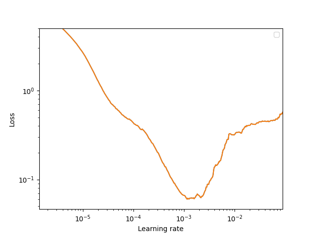
Next, we conduct some learning rate tests to

select a batch size that maximizes GPU utilization on the available hardware and
identify an appropriate learning rate (and potentially weight decay) setting for our dataset and batch size.

This is best done in an interactive session, running the learning rate finder in one window and monitoring the output of nvidia-smi in another.

If you’re running on a SLURM-based cluster, allocate an interactive session with one GPU:

srun --pty --partition=gpu --time=2:00:00 --gres=gpu:1 -c 4 bash
conda activate nfflr
nvidia-smi

+-----------------------------------------------------------------------------+
| NVIDIA-SMI 470.223.02   Driver Version: 470.223.02   CUDA Version: 11.4     |
|-------------------------------+----------------------+----------------------+
| GPU  Name        Persistence-M| Bus-Id        Disp.A | Volatile Uncorr. ECC |
| Fan  Temp  Perf  Pwr:Usage/Cap|         Memory-Usage | GPU-Util  Compute M. |
|                               |                      |               MIG M. |
|===============================+======================+======================|
|   0  Tesla P100-PCIE...  On   | 00000000:5E:00.0 Off |                    0 |
| N/A   37C    P0    26W / 250W |      0MiB / 16280MiB |      0%      Default |
|                               |                      |                  N/A |
+-------------------------------+----------------------+----------------------+
|   1  Tesla P100-PCIE...  On   | 00000000:86:00.0 Off |                    0 |
| N/A   49C    P0    30W / 250W |      0MiB / 16280MiB |      0%      Default |
|                               |                      |                  N/A |
+-------------------------------+----------------------+----------------------+

This session has allocated a single P100 GPU with 16 GiB VRAM. The important fields are the memory utilization and volatile GPU utilization (both at zero here because no code is running on the GPU yet).

assessing GPU utilization#

For a given model configuration, GPU allocation, and batch size, the best training throughput should maximize the utilization of the GPU. Run the learning rate finder, and monitor the output of nvidia-smi to assess the affect of changing the batch size.

nff lr config.py

Note

It’s nice to run these checks with gpustat running in a split-pane tmux window.

gpustat provides a convenient summary of the important GPU utilization stats, and a 100 ms refresh rate typically gives a reasonable idea of the fluctations in GPU utilization.

tmux 
[CTRL-b "]  # split window vertically
python -m gpustat -i 0.1
[CTRL-b o] # switch panes
nff lr config.py

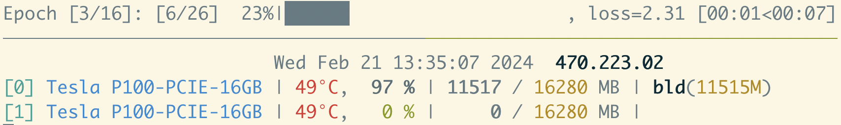
The batch size of 8 that we started with seems reasonable - GPU utilization is consistently around 100 %, and the memory utilization is hovering around 70 % of the available VRAM.

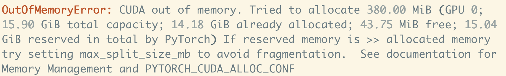
Now that we have this data point, there’s no need to run the learning rate finder to completion at this point. We can try doubling the batch size to 16 - in this case we find the GPU memory limit!

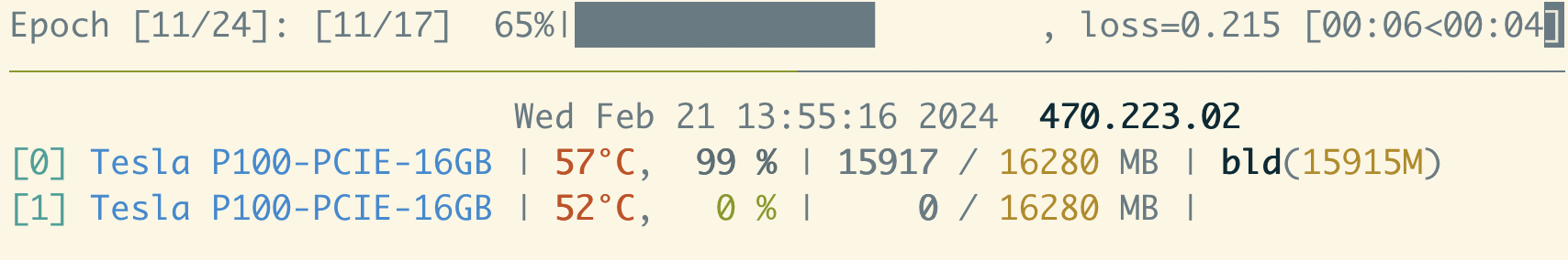
If we back off a bit to a batch size of 12, it seems to be reasonably stable with a memory utilization hovering around 90 % of available VRAM. It’s prudent to leave some head space, especially for datasets with high variability in the number of atoms in the training configurations, which can lead to spikes in memory utilization and out-of-memory woes during production training runs.

Note

If the compute utilization fluctuates a lot (especially if there are bursts of high and low utilization), this likely indicates that the dataloader (or some other CPU-bound process) cannot keep up with the GPU.

Try increasing the number of dataloader workers (4 per GPU is probably a reasonable max) and/or making sure the diskcache setting is configured to use a fast local filesystem. If the workload is still volatile, use the pytorch profiler to identify the bottleneck.

Now that we’ve identified a reasonable batch size that maximizes GPU utilization, run the learning rate test out to completion:

Note

On such a small dataset this exercise is somewhat overkill, since the learning rate finder runs 400 iterations (25 epochs on this training set with a batch size of 12!). However, on large datasets the learning rate finder often completes in a fraction of an epoch.

Based on the learning rate test, let’s choose a peak learning rate of 5e-4. ¹ ¹Running the learning rate finder over a range of weight decay settings can be a reasonable strategy for identifying reasonable settings for both the learning rate and weight decay.

production training run#

After finalizing these settings choices in the configuration file,

full configuration script (config.py)

# config.py
from pathlib import Path
import nfflr

criterion = nfflr.nn.MultitaskLoss(
    tasks=["energy", "forces"],
    weights=[0.5, 0.5]
)

args = nfflr.train.TrainingConfig(
    experiment_dir=Path(__file__).parent.resolve(),
    random_seed=42,
    dataloader_workers=4,
    criterion=criterion,
    epochs=100,
    per_device_batch_size=12,
    weight_decay=1e-3,
    learning_rate=5e-4,
    warmup_steps=0.1,
    diskcache="/tmp/bld",
    initialize_bias=True,
    initialize_estimated_reference_energies=True,
)

rcut = 4.5
transform = nfflr.nn.PeriodicRadiusGraph(cutoff=rcut)
model_cfg = nfflr.models.ALIGNNFFConfig(
    transform=transform,
    cutoff=nfflr.nn.Cosine(rcut),
    local_cutoff=rcut,
    atom_features="embedding",
    reference_energies="trainable",
    alignn_layers=2,
    gcn_layers=2,
    compute_forces=True,
)
model = nfflr.models.ALIGNNFF(model_cfg)

dataset = nfflr.data.mlearn_dataset(
    elements="Si",
    transform=model.transform,
    diskcache=args.diskcache
)

launch a production training run with nff train config.py.

Once the training run completes, you can inspect the loss curves that are written to metric_history.pkl:

/opt/hostedtoolcache/Python/3.10.13/x64/lib/python3.10/site-packages/tqdm/auto.py:21: TqdmWarning: IProgress not found. Please update jupyter and ipywidgets. See https://ipywidgets.readthedocs.io/en/stable/user_install.html
  from .autonotebook import tqdm as notebook_tqdm

2024-03-08 20:07:01,183	INFO util.py:154 -- Missing packages: ['ipywidgets']. Run `pip install -U ipywidgets`, then restart the notebook server for rich notebook output.

2024-03-08 20:07:01,337	INFO util.py:154 -- Missing packages: ['ipywidgets']. Run `pip install -U ipywidgets`, then restart the notebook server for rich notebook output.

---------------------------------------------------------------------------
FileNotFoundError                         Traceback (most recent call last)
Cell In[1], line 12
      9 get_ipython().run_line_magic('matplotlib', 'inline')
     11 modeldir = Path("force-field-training")
---> 12 h = torch.load(modeldir / "metric_history.pkl")
     13 targets = ("loss", "mae_energy", "mae_forces")
     14 n_epochs = len(h["train"][targets[0]])

File /opt/hostedtoolcache/Python/3.10.13/x64/lib/python3.10/site-packages/torch/serialization.py:998, in load(f, map_location, pickle_module, weights_only, mmap, **pickle_load_args)
    995 if 'encoding' not in pickle_load_args.keys():
    996     pickle_load_args['encoding'] = 'utf-8'
--> 998 with _open_file_like(f, 'rb') as opened_file:
    999     if _is_zipfile(opened_file):
   1000         # The zipfile reader is going to advance the current file position.
   1001         # If we want to actually tail call to torch.jit.load, we need to
   1002         # reset back to the original position.
   1003         orig_position = opened_file.tell()

File /opt/hostedtoolcache/Python/3.10.13/x64/lib/python3.10/site-packages/torch/serialization.py:445, in _open_file_like(name_or_buffer, mode)
    443 def _open_file_like(name_or_buffer, mode):
    444     if _is_path(name_or_buffer):
--> 445         return _open_file(name_or_buffer, mode)
    446     else:
    447         if 'w' in mode:

File /opt/hostedtoolcache/Python/3.10.13/x64/lib/python3.10/site-packages/torch/serialization.py:426, in _open_file.__init__(self, name, mode)
    425 def __init__(self, name, mode):
--> 426     super().__init__(open(name, mode))

FileNotFoundError: [Errno 2] No such file or directory: 'force-field-training/metric_history.pkl'

evaluation#

For further evaluation, instantiate a force field model and load the model weights from the final checkpoint file

rcut = 4.5
model_cfg = nfflr.models.ALIGNNFFConfig(
    transform=nfflr.nn.PeriodicRadiusGraph(cutoff=rcut),
    cutoff=nfflr.nn.Cosine(rcut),
    local_cutoff=rcut,
    atom_features="embedding",
    reference_energies="trainable",
    alignn_layers=2,
    gcn_layers=2,
    compute_forces=True,
    energy_units="eV"
)
model = nfflr.models.ALIGNNFF(model_cfg)

model.load_state_dict(
    torch.load(modeldir / "checkpoint_100.pt", map_location="cpu")["model"]
)

<All keys matched successfully>

dataset = nfflr.data.mlearn_dataset("Si", transform=model.transform)

/Users/bld/projects/nfflr/nfflr/atoms.py:84: UserWarning: To copy construct from a tensor, it is recommended to use sourceTensor.clone().detach() or sourceTensor.clone().detach().requires_grad_(True), rather than torch.tensor(sourceTensor).
  self.positions = torch.tensor(positions, dtype=dtype)

The parity plots for both train and validation splits look reasonable:

../_images/fa3de375b034e4eee55ad4f9619ba8031b5d958e95502077956e421615ae691b.png

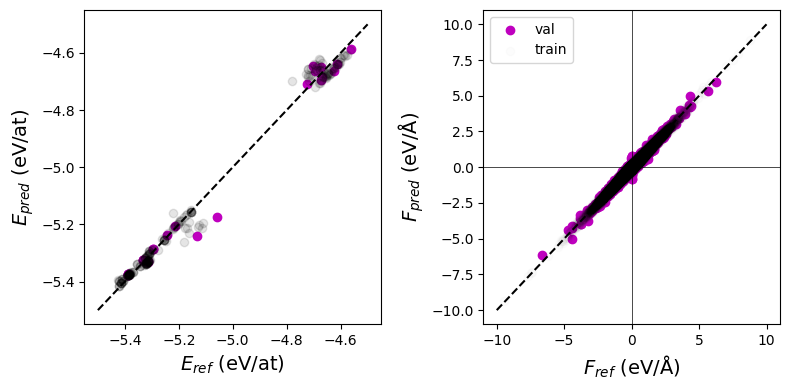
And the mean absolute force errors are around 0.06 eV/Å on the validation set:

torch.mean(torch.abs(pred_t.forces - ref_t.forces))

tensor(0.0456)

torch.mean(torch.abs(pred_v.forces - ref_v.forces))

tensor(0.0645)

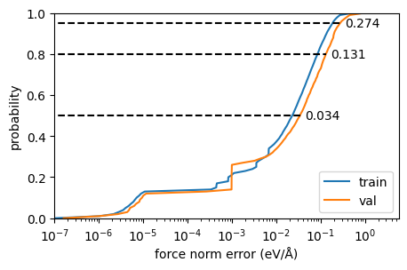
However, force error distributions are often long-tailed, and it helps to inspect the empirical error cumulative distribution for the force magnitudes:

../_images/0b81263f699e18d0945a2996dc1106a13d1fdc9ab6e5c7dfce4ed99178cd6093.png

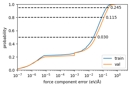
And the raw force components themselves:

../_images/1fd494e8f30cc5d40698a6f6e87f6ca081ffd8ba400292e6d01048ad14de879b.png

Train a force field from scratch

Contents

Train a force field from scratch#

environment#

initial configuration file#

training configuration section#

model section#

dataset section#

tune batch size to maximize GPU utilization#

assessing GPU utilization#

production training run#

evaluation#