8. Scripting and Advanced Features
The analysis can be run from the command line by setting up a Python script. Scripting allows one to build additional analysis tools on top of MOSAIC. The first step is to import MOSAIC as shown below.
import mosaic
Alternatively, one can import sub-modules of MOSAIC directly into a script to access other parts of the system as shown below.
import mosaic.qdfTrajIO as qdf
import mosaic.abfTrajIO as abf

import mosaic.SingleChannelAnalysis
import mosaic.eventSegment as es
import mosaic.adept2State
import mosaic.besselLowpassFilter as bessel
8.1. Import Data and Run an Analysis
Once the required modules are imported, a basic analysis can be run with the code snippet below. The top-level object that is used to configure and run a new analysis is SingleChannelAnalysis, which takes five arguments: i) the path to the data directory, ii) a handle to a TrajIO object that reads in data (e.g. abfTrajIO), iii) a handle to a data filtering algorithm (e.g. besselLowpassFilter or None for no filtering), iv) a handle to a partitioning algorithm (e.g. eventSegment) that partitions the data and v) a handle to a processing algorithm (e.g. adept2State) that processes individual blockade events.
# Process all ABF files in a directory
analysisObj=mosaic.SingleChannelAnalysis.SingleChannelAnalysis(
            '~/ReferenceData/abfSet1',
            abf.abfTrajIO,
            None,
            es.eventSegment,
            moasaic.adept2State.adept2State
        )
The analysis is started by calling the Run() function.
analysisObj.Run()
The code listing above analyzes all ABF files in the specified directory. Handles to trajectory I/O, data filtering, event partitioning and event processing are controlled with their corresponding sections in the Settings File. Default settings used to read ABF files are shown below.
"abfTrajIO" : {
    "filter"            : "*.abf",
    "start"             : 0.0,
    "dcOffset"          : 0.0
}
MOSAIC also supports the QUB QDF file format used by the Electronic Biosciences Nanopatch system. This is accomplished by replacing abfTrajIO in the previous example with qdfTrajIO. Settings for QDF files require two additional parameters to be specified in the settings file, the feedback resistance (Rfb) in Ohms and capacitance (Cfb) in Farads as described in the API Documentation. A sample section of the settings file to read QDF files, followed by Python code required to run an anlysis, is shown below.
"qdfTrajIO": {
        "Rfb"               : 9.1e+12,
        "Cfb"               : 1.07e-12,
        "dcOffset"          : 0.0,
        "filter"            : "*.qdf",
        "start"             : 0.0
    }
# Process all QDF files in a directory
mosaic.SingleChannelAnalysis.SingleChannelAnalysis(
            '~/ReferenceData/qdfSet1',
            qdf.qdfTrajIO,
            None,
            es.eventSegment,
            mosaic.adept2State.adept2State
        ).Run()
Upon completion the analysis writes a log file to the directory containing the data. The log file summarizes the conditions under which the analysis were run, the settings used and timing information.
Start time: 2014-10-05 11:53 AM

[Status]
    Segment trajectory: ***USER STOP***
    Process events: ***NORMAL***


[Summary]
    Baseline open channel conductance:
        Mean    = 136.0 pA
        SD  = 5.5 pA
        Slope   = 0.0 pA/s

    Event segment stats:
        Events detected = 11306

        Open channel drift (max) = 0.0 * SD
        Open channel drift rate (min/max) = (-2.77/3.0) pA/s


[Settings]
    Trajectory I/O settings:
        Files processed = 27
        Data path = ~/ReferenceData/qdfSet1
        File format = qdf
        Sampling frequency = 500.0 kHz

        Feedback resistance = 9.1 GOhm
        Feedback capacitance = 1.07 pF

    Event segment settings:
        Window size for block operations = 0.5 s
        Event padding = 50 points
        Min. event rejection length = 5 points
        Event trigger threshold = 2.36363636364 * SD

        Drift error threshold = 999.0 * SD
        Drift rate error threshold = 999.0 pA/s


    Event processing settings:
        Algorithm = adept2State

        Max. iterations  = 50000
        Fit tolerance (rel. err in leastsq)  = 1e-07
        Blockade Depth Rejection = 0.9


[Output]
    Output path = ~/ReferenceData/qdfSet1
    Event characterization data = ~/ReferenceData/qdfSet1/eventMD-20141005-115324.sqlite
    Event time-series = ***enabled***
    Log file = eventProcessing.log

[Timing]
    Segment trajectory = 98.03 s
    Process events = 0.0 s

    Total = 98.03 s
    Time per event = 8.67 ms
8.1.1. Filter Data
# Filter data with a Bessel filter before processing
mosaic.SingleChannelAnalysis.SingleChannelAnalysis(
            '~/ReferenceData/abfSet1',
            abf.abfTrajIO,
            bessel.besselLowpassFilter,
            es.eventSegment,
            mosaic.adept2State.adept2State
        ).Run()
MOSAIC supports filtering data prior to analysis. This is achieved by passing the dataFilterHnd argument to the SingleChannelAnalysis object. In the code above, the ABF data is filtered using a besselLowpassFilter. Parameters for the filter are defined within the settings file as described in the Settings File section.
"besselLowpassFilter" : {
    "filterOrder"    : "6",
    "filterCutoff"   : "10000",
    "decimate"       : "1"
}
A similar approach can be used to filter data using a waveletDenoiseFilter or a tap delay line (convolutionFilter). Additional filters can be easily added to MOSAIC as described in Extend MOSAIC.
8.2. Advanced Scripting
Scripting with Python allows transforming the output of the MOSAIC further to generate plots, perform additional analysis or extend functionality. Moreover, individual components of the MOSAIC module, which forms the back end code executed in the data processing pipeline, can be used for specific tasks. In this section, we highlight a few typical use cases.
Plot the Ionic Current Time-Series
It is useful to visualize time-series data to highlight unique characteristics of a sample. For example the sample code above was used to load 1 second of monodisperse PEG28 data, sampled at 500 kHz. The data was read using a abfTrajIO object similar to the examples above. The popdata() command was used to take 500k data points (or 1 second) and then plot a time-series using matplotlib (see figure below). Calling popdata() again will return the next n points.
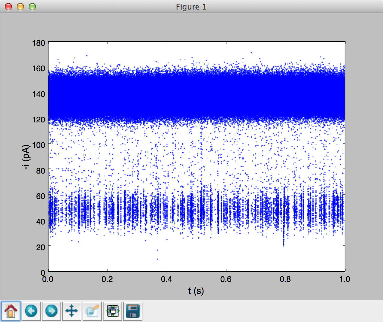
We have packaged time-series plotting into an easy to use module timeseries. Run interactive examples in an IPython notebook: |timeseries|
Estimate the Channel Gating Duration
Scripting can be used to obtain statistics from the raw time-series. In the code snippet below, we estimate the amount of time a channel spends in a gated state by combining modules defined within MOSAIC. The analysis is performed in blocks for efficiency. We first define a Python function that takes multiple arguments including TrajIO object, the threshold at which we want to define the gated state in pA (gatingcurrentpa), the block size in seconds (blocksz), the total time of the time-series being processed in seconds (totaltime) and the sampling rate of the data in Hz (fshz). The function then calculates the number of blocks in which the channel was in a gated state and returns the time spent in that state in seconds.
Plot the Output of an Analysis
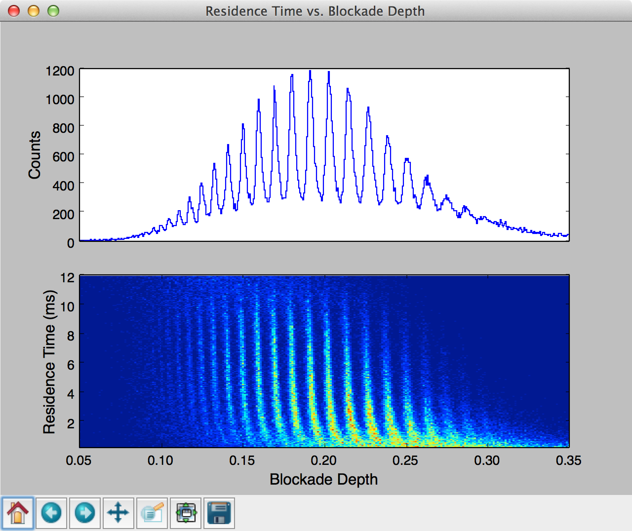
This final example shows how one can use MOSAIC to process an ionic current time-series and then build a custom script that further analyses and plots the results. This example uses single-molecule mass spectrometry (SMMS) data [], described in more detail in the Single Molecule Mass Spectrometry section .
In the code below, we first process all the ABF files in a specified directory similar to the examples in previous sections. Upon completion of the analysis, the results are stored in a SQLite database, which can be then queried using the structured query language (SQL).
Running the code above generates a two pane plot using matplotlib. The top pane contains a histogram of the blockade depth, while the bottom pane plots a 2D histogram of residence time vs. blockade depth.