Why tmmc-lnpy?#
Note
While the distribution is named tmmc-lnpy, it provides the python package lnpy. This naming was done to avoid conflicts with other packages on pypi. The name of the module lnpy may be changed in the future.
lnpy is a python package to analyze the main output of Grand Canonical Transition Matrix Monte Carlo (GC-TMMC) simulations: \(\ln \Pi(N)\). Hence the name. lnpy is designed to calculate a host of properties in the Canonical and Grand Canonical ensembles. For a review of GC-TMMC and the property \(\ln \Pi(N)\), look at some of the following references:
Direct evaluation of multicomponent phase equilibria using flat-histogram methods
Direct calculation of liquid–vapor phase equilibria from transition matrix Monte Carlo simulation
\(\Pi(N; \mu, T, V)\) is the macrostate probability of observing \(N\) particles at a given chemical potential \(\mu\), temperature \(T\) and volume \(V\). We drop the explicit mention of \(\mu\), \(V\) and \(T\) below for simplicity. This distribution is related to the grand canonical ensemble by:
Where \(\beta = 1 / (k_{\rm B} T)\) is the inverse temperature, \(k_{\rm B}\) is Boltzmann’s constant, \(Q(N, V, T)\) is the canonical partition function, and \(\Xi(\mu, V, T)\) is the grand canonical partition function. GC-TMMC simulation provide a means to calculate the \(\ln \Pi(N; \mu, V, T)\) directly. One of the truly excellent qualities of such simulations is that once \(\ln \Pi\) is collected at a given chemical potential \(\mu_0\), it can be rescaled to any other chemical potential \(\mu\) through rescaling of the form:
where \(C\) is a normalization constant which does not effect most calculated properties. From \(\ln \Pi(N)\), many thermodynamic properties can be calculated. The grand potential \(\Omega\), and hence the system pressure \(p\), can be obtained from
Also, grand canonical averages can be calculated from canonical averages using \(\ln \Pi(N)\):
Plus, \(\ln \Pi\) can be directly analyzed to identify unique phases, phase transitions, limits of stability, etc. The package lnpy provides a simple means to perform all the above calculations simply, and quickly.
Usage#
Lets consider a simple example: a Lennard-Jones (LJ) fluid at supercritical temperatures.
An example value of \(\ln \Pi(N)\) (shortened to lnPi) can be loaded directly from lnpy package:
import numpy as np

import lnpy.examples

data_dict = lnpy.examples.load_example_dict("lj_sup")
with np.printoptions(precision=2, suppress=True, threshold=5):
    for k, v in data_dict.items():
        print(f"{k}:{v!r}")
lnPi_data:array([-1559.75, -1550.74, -1542.43, ...,   -10.01,   -11.02,   -12.08])
lnPi_mask:array([False, False, False, ..., False, False, False])
state_kws:{'beta': 0.6666666666666666, 'volume': 512.0}
extra_kws:{'PE': array([    0.  ,     0.  ,    -0.02, ..., -1643.18, -1648.71, -1654.36])}
lnz:array([2.77])
Here, we have the parameters
lnPi_data: the actual value of \(\ln \Pi(N)\).
lnPi_mask: bool array. where
mask == True, values are ‘masked out’state_kws: dict of ‘state’ variables. Here, it include the inverse temperature ‘beta’ \(=\beta = 1/(k_{\rm B} T)\) and the systems volume ‘volume’ \(=V\)
extra_kws: dict of ‘extra’ variables. Here, it include ‘PE’, the canonical potential energy
lnz: log of activity \(\ln z = \beta \mu\), where \(\mu\) is chemical potential.
lnPiMasked#
The first important class is lnPiMasked. This class handles the basics of dealing with \(\ln \Pi(N)\). To create it, to the following.
%matplotlib inline
import matplotlib.pyplot as plt

ref = lnpy.lnPiMasked.from_data(
    lnz=data_dict["lnz"],
    lnz_data=data_dict["lnz"],
    data=data_dict["lnPi_data"],
    mask=data_dict["lnPi_mask"],
    state_kws=data_dict["state_kws"],
    extra_kws=data_dict["extra_kws"],
)
ref
<lnPi(lnz=[2.76512052])>
To access the underlying data, use the following
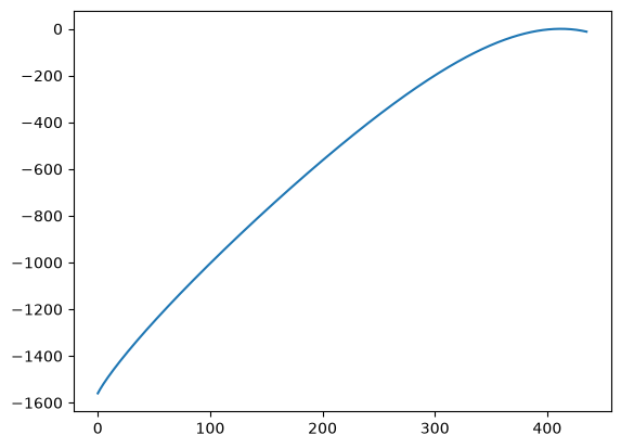
plt.plot(ref.data)
[<matplotlib.lines.Line2D at 0x7febf25d5450>]
Reweighting results#
One of the amazing things about \(\ln \Pi(N)\) calculated at some chemical potential \(\mu_{\rm ref}\) is that it can be reweighted to any other chemical potential \(\mu\). This is done with the formula
To reweight data to another value of \(\ln z\), we use the lnpy.lnpidata.lnPiMasked.reweight() method:
new = ref.reweight(4.0)
print(new)
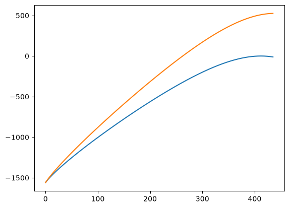
# compare to original
plt.plot(ref.data, label=ref.lnz)
plt.plot(new.data, label=new.lnz)
<lnPi(lnz=[4.])>
[<matplotlib.lines.Line2D at 0x7febf23fe850>]
lnpy.lnpidata.lnPiMasked has a variety of utilities to work with the \(\ln \Pi(N)\) data. For example
zeromax: shift \(\ln \Pi(N)\) such that maximum value is zero. Useful for numerical stability
ma :
MaskedArrayview of data. Used when constructing phases, and working with multicomponent data.
Check out the api docs for further details
Calculating Ensemble properties#
\(\ln \Pi(N)\) can be used to calculate a variety of properties in the Canonical and Grand Canonical ensembles.
To make everything easier, the actual value of \(\ln \Pi(N)\) is wrapped in an DataArray object, which provides some nice data goodies. To access this view, use the xce or xge accessors (short for Xarray Canonical Ensemble and Xarray Grand canonical Ensemble). For example, the canonical properties can be obtained as follows:
Note
We only show a small subset of functionality. For further information, see lnPiMasked.
# pressure
ref.xce.pressure().head()
<xarray.DataArray 'pressure' (n_0: 5)> Size: 40B
array([-0.        ,  0.00100796,  0.00319043,  0.00560728,  0.00813105])
Coordinates:
  * n_0      (n_0) int64 40B 0 1 2 3 4
    beta     float64 8B 0.6667
    volume   float64 8B 512.0
Attributes:
    dims_n:      ['n_0']
    dims_lnz:    ['lnz_0']
    dims_comp:   ['component']
    dims_state:  ['lnz_0', 'beta', 'volume']
long_name: $p({\bf n},V,T)$# scaled Helmholtz free energy
ref.xce.betaF().head()
<xarray.DataArray 'betaF' (n_0: 5)> Size: 40B
array([  0.        ,  -6.23817948, -11.78825896, -16.93743845,
       -21.80391793])
Coordinates:
  * n_0      (n_0) int64 40B 0 1 2 3 4
    beta     float64 8B 0.6667
    volume   float64 8B 512.0
Attributes:
    dims_n:         ['n_0']
    dims_lnz:       ['lnz_0']
    dims_comp:      ['component']
    dims_state:     ['lnz_0', 'beta', 'volume']
    standard_name:  helmholtz_free_energy
long_name: $\beta F({\bf n},V,T)$Look at the documentation for all the properties available. To quickly construct a dataset of multiple properties, use the table method.
ds = ref.xce.table(keys=["pressure", "betaF"], default_keys=None)
ds
<xarray.Dataset> Size: 10kB
Dimensions:   (n_0: 436)
Coordinates:
  * n_0       (n_0) int64 3kB 0 1 2 3 4 5 6 7 ... 429 430 431 432 433 434 435
    beta      float64 8B 0.6667
    volume    float64 8B 512.0
Data variables:
    pressure  (n_0) float64 3kB -0.0 0.001008 0.00319 ... 5.786 5.854 5.893
    betaF     (n_0) float64 3kB 0.0 -6.238 -11.79 ... -352.4 -348.7 -344.8
Attributes:
    dims_n:      ['n_0']
    dims_lnz:    ['lnz_0']
    dims_comp:   ['component']
    dims_state:  ['lnz_0', 'beta', 'volume']
long_name: $p({\bf n},V,T)$This can be easily converted to a pandas.DataFrame
ds.to_dataframe().head()
| beta | volume | pressure | betaF | |
|---|---|---|---|---|
| n_0 | ||||
| 0 | 0.666667 | 512.0 | -0.000000 | 0.000000 |
| 1 | 0.666667 | 512.0 | 0.001008 | -6.238179 |
| 2 | 0.666667 | 512.0 | 0.003190 | -11.788259 |
| 3 | 0.666667 | 512.0 | 0.005607 | -16.937438 |
| 4 | 0.666667 | 512.0 | 0.008131 | -21.803918 |
To access Grand Canonical properties, use the xge accessor
ref.xge.pressure()
<xarray.DataArray 'pressure' ()> Size: 8B
array(4.57687966)
Coordinates:
    lnz_0    float64 8B 2.765
    beta     float64 8B 0.6667
    volume   float64 8B 512.0
Attributes:
    dims_n:         ['n_0']
    dims_lnz:       ['lnz_0']
    dims_comp:      ['component']
    dims_state:     ['lnz_0', 'beta', 'volume']
    standard_name:  grand_potential
long_name: $p(\mu,V,T)$ref.xge.betaF()
<xarray.DataArray 'betaF' ()> Size: 8B
array(-423.16867869)
Coordinates:
    lnz_0    float64 8B 2.765
    beta     float64 8B 0.6667
    volume   float64 8B 512.0
Attributes:
    dims_n:         ['n_0']
    dims_lnz:       ['lnz_0']
    dims_comp:      ['component']
    dims_state:     ['lnz_0', 'beta', 'volume']
    standard_name:  helmholtz_free_energy
long_name: $\beta F(\mu,V,T)$Or, to calculate multiple properties, again, use the table method
ref.xge.table(keys=["pressure", "betaF"], default_keys=None)
<xarray.Dataset> Size: 40B
Dimensions:   ()
Coordinates:
    lnz_0     float64 8B 2.765
    beta      float64 8B 0.6667
    volume    float64 8B 512.0
Data variables:
    pressure  float64 8B 4.577
    betaF     float64 8B -423.2
Attributes:
    dims_n:         ['n_0']
    dims_lnz:       ['lnz_0']
    dims_comp:      ['component']
    dims_state:     ['lnz_0', 'beta', 'volume']
    standard_name:  grand_potential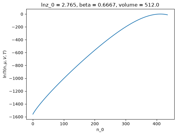
long_name: $p(\mu,V,T)$The great thing about using the xarray interface is that things like plotting become trivial. For example, use
ref.xge.lnpi().plot()
[<matplotlib.lines.Line2D at 0x7febf22d1090>]
Collections of lnPi Values#
Ok, we can reweight a \(\ln \Pi(N)\) from one chemical potential to another, and calculate a variety of properties for a \(\ln \Pi(N)\). But what if we want to calculate properties at a variety of values of \(\ln z\). We could do list comprehension, but that’s slow, and can get unwieldy. Instead, lnpy provides a helper class to deal with multiple lnPis. To use it, we must first have a PhaseCreator object. We will discuss this object in detail later, but for now, know that for the simple case of a single component system that does not have any phase transitions, it suffices to use the following.
phase_creator = lnpy.PhaseCreator(nmax=1, ref=ref)

build_phases = phase_creator.build_phases_mu([None])
To create a collection of with of lnPi at different values of lnz, use the lnpy.lnpiseries.lnPiCollection class:
with lnpy.set_options(tqdm_leave=True):
    c = lnpy.lnPiCollection.from_builder(
        lnzs=np.linspace(-10, 3, 2000), build_phases=build_phases
    )
lnPiCollection is a wrapper around pandas.Series. This provides an index for each lnPiMasked instance. This
allows some niceties like indexing by value, groupby, etc.
# Select by position
# scalar index gives object
c.iloc[1]
<lnPi(lnz=[-9.99349675])>
# array-like gives lnPiCollection instance
(c.iloc[[1]])
<class lnPiCollection>
lnz_0      phase
-9.993497  0        [-9.993496748374188]
dtype: object
# select by value.  Same as indexing into pandas.Series
c.loc[[3.0]]
<class lnPiCollection>
lnz_0  phase
3.0    0        [3.0]
dtype: object
# can also query
c.query("lnz_0 > 2.95")
<class lnPiCollection>
lnz_0     phase
2.954477  0         [2.95447723861931]
2.960980  0        [2.960980490245122]
2.967484  0        [2.967483741870936]
2.973987  0        [2.973986993496748]
2.980490  0        [2.980490245122562]
2.986993  0        [2.986993496748374]
2.993497  0        [2.993496748374188]
3.000000  0                      [3.0]
dtype: object
Accessing properties of collection#
The really nice thing about lnPiCollection is that all the properties for all the lnPiMasked objects can be calculated at once, in a vectorized way. The same accessor xge is available to lnPiCollection as for lnPiMasked. Note that the xce accessor is not available, as it only makes sense for a single value of lnPiMasked.
# Note the smart indexing.  The index is inherited from lnPiCollection.index
c.xge.pressure()
<xarray.DataArray 'pressure' (lnz_0: 2000, phase: 1)> Size: 16kB
array([[6.80940123e-05],
       [6.85383141e-05],
       [6.89855151e-05],
       ...,
       [4.84631185e+00],
       [4.85425839e+00],
       [4.86220769e+00]])
Coordinates:
  * lnz_0    (lnz_0) float64 16kB -10.0 -9.993 -9.987 -9.98 ... 2.987 2.993 3.0
  * phase    (phase) int64 8B 0
    beta     float64 8B 0.6667
    volume   float64 8B 512.0
Attributes:
    dims_n:         ['n_0']
    dims_lnz:       ['lnz_0']
    dims_comp:      ['component']
    dims_state:     ['lnz_0', 'beta', 'volume']
    dims_rec:       ['sample']
    standard_name:  grand_potential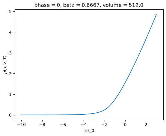
long_name: $p(\mu,V,T)$# plot the results
c.xge.pressure().plot()
[<matplotlib.lines.Line2D at 0x7febe9cc96d0>]
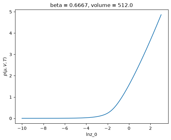
This is much more convenient (and much faster) than doing something like:
# Don't do things like this
# It's super slow
import xarray as xr

pressures = [x.xge.pressure() for x in c]

xr.concat(pressures, dim="lnz_0").plot()
[<matplotlib.lines.Line2D at 0x7febe9cfbc50>]
Loading examples#
lnPi comes with some pre-defined examples in the examples module. We used it above to load a dictionary of data that we then turned into a lnPiMasked object. This can be streamlined using the following:
import lnpy.examples

ref = lnpy.examples.load_example_lnpimasked("lj_sup")
ref
<lnPi(lnz=[2.76512052])>
Alternatively, for some examples, you can load an object with contains a predefined PhaseCreator object. We’ll save this for later.
Single component system with phase transitions.#
Next, let’s consider a system with a phase transition. First, lets load some example data
%matplotlib inline
import matplotlib.pyplot as plt
import numpy as np
import xarray as xr

import lnpy
import lnpy.examples

# Subcritical LJ data
ref = lnpy.examples.load_example_lnpimasked("lj_sub")
# look at the lnPi values
ref.xge.lnpi().plot()
[<matplotlib.lines.Line2D at 0x7febe8bae710>]
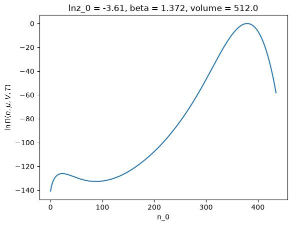
Notice that this \(\ln \Pi(N)\) has multiple maxima. This indicates that multiple phases coexist.
So calculating properties from the total lnPiMasked doesn’t make sense. Instead, the lnPiMasked should be divided into phases. The division should be at the local minima in \(\ln \Pi(N)\) (at approximately n_0=100 in the example above). To perform the segmentation, we turn back to the PhaseCreator object. Let see how this works
# This creates a `PhaseCreator` object
phase_creator = lnpy.PhaseCreator(nmax=2, nmax_peak=4, ref=ref, merge_kws={"efac": 0.8})
# call the `build_phases` method creates a lnPiCollection of phases
p = phase_creator.build_phases()
p
<class lnPiCollection>
lnz_0      phase
-3.609956  0        [-3.6099564097351307]
           1        [-3.6099564097351307]
dtype: object
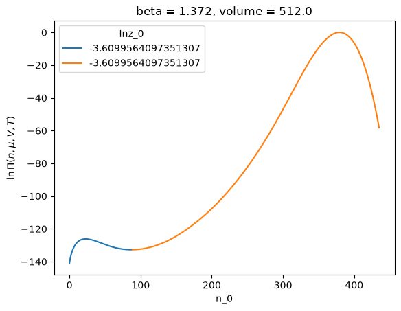
# plot the lnpi values for each 'phase'
p.xge.lnpi().plot(hue="lnz_0")
[<matplotlib.lines.Line2D at 0x7febe8abee90>,
 <matplotlib.lines.Line2D at 0x7febe8abefd0>]
What just happened? To segment \(\ln \Pi(N)\) the code does the following:, we For this we do the following
Find the local maxima of the \(\ln \Pi(N)\). This is done using
peak_local_max_adaptive(), which is an an adaptive version ofskimage.feature.peak_local_max(). This finds at mostnmax_peak. Note thatnmax_peakcan be any number.Use the
watershed()segmentation algorithm to segment \(-\ln \Pi\) into regions about the local minima in \(-\ln \Pi\) (local maxima in \(\ln \Pi\)).Remove any phases that have to low a transition energy. We discuss this further below.
If the number of ‘phases’ is greater than the maximum allowed number of phases. Merge them. This is done by analyzing the transition energy between phases. Discussed further below.
Merge phases that have same
phase_id. Discussed further below.Pass list of
lnPiMaskedobjects and createdindextophases_factoryfunction. Discussed further below.return result
OK, that’s a bunch of steps. Let take them one at a time.
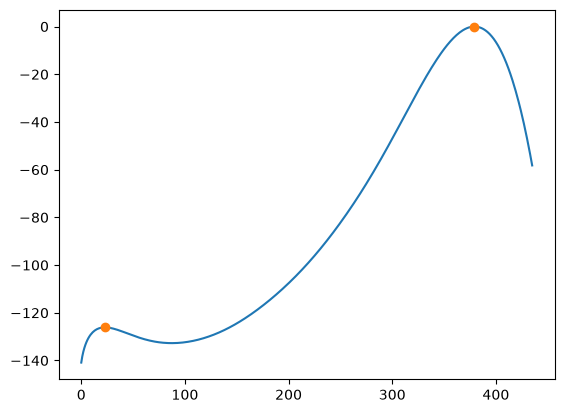
Local maxima#
maxima_marker = lnpy.segment.peak_local_max_adaptive(
    ref.data, num_peaks_max=4, mask=~ref.mask, style="marker"
)
maxima_index = np.where(maxima_marker > 0)
plt.plot(ref.data)
plt.plot(maxima_index[0], ref.data[maxima_index], marker="o", ls="None")
[<matplotlib.lines.Line2D at 0x7febf46a2490>]
Watershed#
OK, great. Now we can segment the data. lnPi provides a wrapper to skimage.segmentation.watershed() through lnpy.segment.Segmenter.watershed().
s = lnpy.segment.Segmenter()
labels = s.watershed(-ref.data, markers=maxima_marker, mask=~ref.mask)
labels
array([1, 1, 1, 1, 1, 1, 1, 1, 1, 1, 1, 1, 1, 1, 1, 1, 1, 1, 1, 1, 1, 1,
       1, 1, 1, 1, 1, 1, 1, 1, 1, 1, 1, 1, 1, 1, 1, 1, 1, 1, 1, 1, 1, 1,
       1, 1, 1, 1, 1, 1, 1, 1, 1, 1, 1, 1, 1, 1, 1, 1, 1, 1, 1, 1, 1, 1,
       1, 1, 1, 1, 1, 1, 1, 1, 1, 1, 1, 1, 1, 1, 1, 1, 1, 1, 1, 1, 1, 1,
       2, 2, 2, 2, 2, 2, 2, 2, 2, 2, 2, 2, 2, 2, 2, 2, 2, 2, 2, 2, 2, 2,
       2, 2, 2, 2, 2, 2, 2, 2, 2, 2, 2, 2, 2, 2, 2, 2, 2, 2, 2, 2, 2, 2,
       2, 2, 2, 2, 2, 2, 2, 2, 2, 2, 2, 2, 2, 2, 2, 2, 2, 2, 2, 2, 2, 2,
       2, 2, 2, 2, 2, 2, 2, 2, 2, 2, 2, 2, 2, 2, 2, 2, 2, 2, 2, 2, 2, 2,
       2, 2, 2, 2, 2, 2, 2, 2, 2, 2, 2, 2, 2, 2, 2, 2, 2, 2, 2, 2, 2, 2,
       2, 2, 2, 2, 2, 2, 2, 2, 2, 2, 2, 2, 2, 2, 2, 2, 2, 2, 2, 2, 2, 2,
       2, 2, 2, 2, 2, 2, 2, 2, 2, 2, 2, 2, 2, 2, 2, 2, 2, 2, 2, 2, 2, 2,
       2, 2, 2, 2, 2, 2, 2, 2, 2, 2, 2, 2, 2, 2, 2, 2, 2, 2, 2, 2, 2, 2,
       2, 2, 2, 2, 2, 2, 2, 2, 2, 2, 2, 2, 2, 2, 2, 2, 2, 2, 2, 2, 2, 2,
       2, 2, 2, 2, 2, 2, 2, 2, 2, 2, 2, 2, 2, 2, 2, 2, 2, 2, 2, 2, 2, 2,
       2, 2, 2, 2, 2, 2, 2, 2, 2, 2, 2, 2, 2, 2, 2, 2, 2, 2, 2, 2, 2, 2,
       2, 2, 2, 2, 2, 2, 2, 2, 2, 2, 2, 2, 2, 2, 2, 2, 2, 2, 2, 2, 2, 2,
       2, 2, 2, 2, 2, 2, 2, 2, 2, 2, 2, 2, 2, 2, 2, 2, 2, 2, 2, 2, 2, 2,
       2, 2, 2, 2, 2, 2, 2, 2, 2, 2, 2, 2, 2, 2, 2, 2, 2, 2, 2, 2, 2, 2,
       2, 2, 2, 2, 2, 2, 2, 2, 2, 2, 2, 2, 2, 2, 2, 2, 2, 2, 2, 2, 2, 2,
       2, 2, 2, 2, 2, 2, 2, 2, 2, 2, 2, 2, 2, 2, 2, 2, 2, 2], dtype=int32)
Each unique value in labels corresponds to a phase. We can construct multiple lnPiMasked objects from labels using
local free energy#
Now, we look at the local free energy. The local (scaled) free energy is defined as \(w(N) = \beta f(N) = -\ln \Pi(N)\). We consider the energy at the location of the local minima in \(w\) (local maxima in \(\ln \Pi\)) versus the value of \(w\) at the transition between phases (around \(n=100\) in the figure above). This is performed by the class lnpy.lnpienergy.wFreeEnergy.
from lnpy.lnpienergy import wFreeEnergy
w = wFreeEnergy.from_labels(data=ref.data, labels=labels)
# this is the same as -lnPi[maxima]
w.w_min
array([[126.12754742],
       [ -0.        ]])
-ref.data[maxima_index]
array([126.12754742, -0. ])
# w.w_tran[i, j] is the 'transition' energy going from phase i to phase j
w.w_tran
array([[         inf, 132.72931142],
       [132.72931142,          inf]])
# the transition between phases '0' and '1' is at index 87
w.w_argtran
{(0, 1): (87,)}
-ref.data[87]
132.72931142169
# the change in energy between the phases
w.delta_w
array([[         inf,   6.601764  ],
       [132.72931142,          inf]])
This transition energy means the two phases are stable. So move on.
lnpis = ref.list_from_masks(w.masks)
lnpis
[<lnPi(lnz=[-3.60995641])>, <lnPi(lnz=[-3.60995641])>]
Construct collection#
Now these can be converted to a lnPiCollection object.
p = lnpy.lnPiCollection.from_list(lnpis, index=[0, 1])
p
<class lnPiCollection>
lnz_0      phase
-3.609956  0        [-3.6099564097351307]
           1        [-3.6099564097351307]
dtype: object
So, the segmentation can get pretty involved. This is why there is the helper class PhaseCreator. There are a slew
of options to the different routines. Look at the docs for more information
At a different \(\ln z\) value#
Let us instead consider a different value of chemical potential. One near the critical point.
p = phase_creator.build_phases(-3.49)
p
<class lnPiCollection>
lnz_0  phase
-3.49  0        [-3.49]
       1        [-3.49]
dtype: object
p.xge.lnpi().plot(hue="phase")
[<matplotlib.lines.Line2D at 0x7febe8cbccd0>,
 <matplotlib.lines.Line2D at 0x7febe8cbce10>]
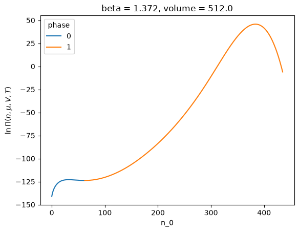
But lets look at the local free energy ‘w’ defined above. This can be obtained by the accessor wfe in lnPiCollection.
# min(w) in each phase
p.wfe.w_min
lnz_0  phase
-3.49  0        122.930891
       1        -45.776165
Name: w_min, dtype: float64
# transition w from phase to phase_nebr
p.wfe.w_tran
lnz_0  phase  phase_nebr
-3.49  0      0                    inf
              1             123.785912
       1      0             123.785912
              1                    inf
Name: w_tran, dtype: float64
# w_tran - w_min
p.wfe.dw
lnz_0  phase  phase_nebr
-3.49  0      0                    inf
              1               0.855021
       1      0             169.562078
              1                    inf
Name: delta_w, dtype: float64
We see that the \(\Delta w\) is pretty low at this value of \(\ln z\). We passed in the parameter efac=0.8 in the definition of phase_creator. If we instead wish to remove phases with an energy this low, we can do the following:
p = phase_creator.build_phases(-3.49, efac=0.9)
p
<class lnPiCollection>
lnz_0  phase
-3.49  0        [-3.49]
dtype: object
Now if the \(\Delta w\) between phases is smaller than efac, the phases are merged. For more information, see that api docs.
Tagging phases#
PhaseCreator allows passing a callback tag_phases to attach a label to each phase. By default, the phases are labeled by there list index. This can be confusing, because over a range of \(\ln z\) values, different physical phases can have the same label. For example
phase_creator = lnpy.PhaseCreator(nmax=2, nmax_peak=4, ref=ref, merge_kws={"efac": 0.8})
c = lnpy.lnPiCollection.from_builder(
    np.linspace(-10, -2, 50), build_phases=phase_creator.build_phases
)

# this looks weird because have multiple phases and not sure which is which
c.xge.pressure().plot(hue="phase")
[<matplotlib.lines.Line2D at 0x7febe876d6d0>,
 <matplotlib.lines.Line2D at 0x7febe876d810>]
Note that this can be fixed by considering ‘stable’ phases only
(
    c.xge
    .table(["mask_stable", "pressure"], default_keys=None)
    .assign(pressure_stable=lambda x: x["pressure"].where(x["mask_stable"]))
    .pressure_stable.max("phase")
    .plot()
)
[<matplotlib.lines.Line2D at 0x7febe8822e90>]
There are two clear phases here. It would be beneficial to label the liquid and vapor phases differently. So we define the callback tag_phases
def tag_phases(list_of_phases):
    """
    Simple tag_phases callback

    This looks at the local maximum of each lnPiMasked object.

    If location of maximum < len(data)/2 -> phase = 0
    else -> phase = 1

    """
    if len(list_of_phases) > 2:
        msg = "bad tag function"
        raise ValueError(msg)
    argmax0 = np.array([xx.local_argmax()[0] for xx in list_of_phases])
    return np.where(argmax0 <= list_of_phases[0].shape[0] / 2, 0, 1)
phase_creator = lnpy.PhaseCreator(
    nmax=2, nmax_peak=4, ref=ref, merge_kws={"efac": 0.8}, tag_phases=tag_phases
)
c = lnpy.lnPiCollection.from_builder(
    np.linspace(-10, -2, 50), build_phases=phase_creator.build_phases
)

c.xge.pressure().plot(hue="phase")
[<matplotlib.lines.Line2D at 0x7febe89f9d10>,
 <matplotlib.lines.Line2D at 0x7febe89f9e50>]
Calculation Binodal and spinodal#
The binodal and spinodal can be found using the lnpy.stability module. This module adds accessors to lnPiCollection class. A collection is needed to provide a decent guess for the location of the binodal and spinodal.
# must import stability to add the accessors to lnPiCollection
import lnpy.stability
%matplotlib inline
import matplotlib.pyplot as plt
import numpy as np
import xarray as xr

import lnpy
import lnpy.examples

# Subcritical LJ data
ref = lnpy.examples.load_example_lnpimasked("lj_sub")

phase_creator = lnpy.PhaseCreator(
    nmax=2, nmax_peak=4, ref=ref, merge_kws={"efac": 0.8}, tag_phases=tag_phases
)

# Here we need a scalar builder object.
build_phases = phase_creator.build_phases_mu([None])
# initial guess
c = lnpy.lnPiCollection.from_builder(
    np.linspace(-10, -2, 10), build_phases=phase_creator.build_phases_mu([None])
)
The spinodal is calculates as the location where \(\Delta w\) equals some value. Lets say we want to define the spinodal as the location where \(\Delta w = 1.0\). We do the following:
_ = c.spinodal(
    phase_ids=2,  # the id's of the phases we're considering
    build_phases=phase_creator.build_phases_mu([None]),
    # this is the efac parameter for
    build_kws={"efac": 0.5},
    inplace=True,
    as_dict=False,
    efac=1.0,
)
# to access the data as a collection, use the `access` attribute
c.spinodal.access
<class lnPiCollection>
spinodal  lnz_0      phase
0         -3.494734  0        [-3.494734034735128]
                     1        [-3.494734034735128]
1         -4.379828  0        [-4.379828176267564]
                     1        [-4.379828176267564]
dtype: object
# energetics
# spinodal 0 is the limit of stability for phase 0 -> phase 1
# spinodal 1 is the limit of stability for phase 1 -> phase 0
c.spinodal.access.wfe.dw
spinodal  lnz_0      phase  phase_nebr
0         -3.494734  0      0                    inf
                            1               1.000000
                     1      0             168.038523
                            1                    inf
1         -4.379828  0      0                    inf
                            1             142.179651
                     1      0               1.000000
                            1                    inf
Name: delta_w, dtype: float64
Now that we have the spinodal, we can calculation the binodal
bino = c.binodal(
    phase_ids=[0, 1],
    build_phases=phase_creator.build_phases_mu([None]),
    build_kws={"efac": 0.5},
    inplace=True,
)
# access as collection with the `access` attribute
c.binodal.access
<class lnPiCollection>
binodal  lnz_0      phase
0        -3.966438  0        [-3.966438059499727]
                    1        [-3.966438059499727]
dtype: object
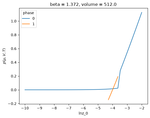
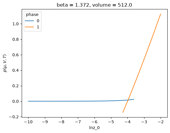
# at the binodal, the two phases should have equal pressure
c.binodal.access.xge.pressure()
<xarray.DataArray 'pressure' (binodal: 1, lnz_0: 1, phase: 2)> Size: 16B
array([[[0.01594237, 0.01594237]]])
Coordinates:
  * binodal  (binodal) int64 8B 0
  * lnz_0    (lnz_0) float64 8B -3.966
  * phase    (phase) int64 16B 0 1
    beta     float64 8B 1.372
    volume   float64 8B 512.0
Attributes:
    dims_n:         ['n_0']
    dims_lnz:       ['lnz_0']
    dims_comp:      ['component']
    dims_state:     ['lnz_0', 'beta', 'volume']
    dims_rec:       ['sample']
    standard_name:  grand_potential
long_name: $p(\mu,V,T)$To append spinodal/binodal to the dataset, use the following:
c_total = c.append(c.spinodal.appender).append(c.binodal.appender)
c_total
<class lnPiCollection>
lnz_0       phase
-10.000000  0                      [-10.0]
-9.111111   0          [-9.11111111111111]
-8.222222   0         [-8.222222222222221]
-7.333333   0         [-7.333333333333334]
-6.444444   0         [-6.444444444444445]
-5.555556   0         [-5.555555555555555]
-4.666667   0         [-4.666666666666667]
-3.777778   0        [-3.7777777777777786]
            1        [-3.7777777777777786]
-2.888889   1        [-2.8888888888888893]
-2.000000   1                       [-2.0]
-3.494734   0         [-3.494734034735128]
            1         [-3.494734034735128]
-4.379828   0         [-4.379828176267564]
            1         [-4.379828176267564]
-3.966438   0         [-3.966438059499727]
            1         [-3.966438059499727]
dtype: object
and if you’d like to sort the index:
c_total.sort_index()
<class lnPiCollection>
lnz_0       phase
-10.000000  0                      [-10.0]
-9.111111   0          [-9.11111111111111]
-8.222222   0         [-8.222222222222221]
-7.333333   0         [-7.333333333333334]
-6.444444   0         [-6.444444444444445]
-5.555556   0         [-5.555555555555555]
-4.666667   0         [-4.666666666666667]
-4.379828   0         [-4.379828176267564]
            1         [-4.379828176267564]
-3.966438   0         [-3.966438059499727]
            1         [-3.966438059499727]
-3.777778   0        [-3.7777777777777786]
            1        [-3.7777777777777786]
-3.494734   0         [-3.494734034735128]
            1         [-3.494734034735128]
-2.888889   1        [-2.8888888888888893]
-2.000000   1                       [-2.0]
dtype: object
Multi component systems#
lnPi is designed to work with single and multicomponent systems. Let’s take a look at a system without phase transitions to start.
import lnpy.examples
data = lnpy.examples.load_example_dict("ljmix_sup")
f, a = plt.subplots(figsize=(4, 4))
a.imshow(data["lnPi_data"])
<matplotlib.image.AxesImage at 0x7febe8ee1550>
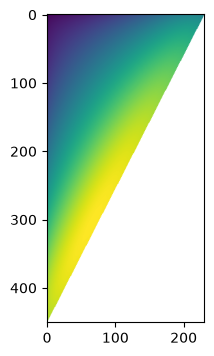
We have finite data along the upper corner of the matrix ‘lnPi_data’. Therefore, the base lnPiMasked object, without splitting into phases, also will have a mask. This is why everything was build up from the numpy.ma.MaskedArray class.
data
{'lnPi_data': array([[-759.26449941, -756.19423037, -753.77081946, ..., -424.28411489,
         -425.66274776, -426.93571412],
        [-755.52637941, -752.42375982, -749.96557613, ..., -418.59148639,
         -419.73805248,           nan],
        [-752.45715941, -749.31971691, -746.82151608, ..., -413.26963103,
         -414.54424182,           nan],
        ...,
        [-104.40479985, -102.4117824 ,           nan, ...,           nan,
                   nan,           nan],
        [-105.98668385,           nan,           nan, ...,           nan,
                   nan,           nan],
        [-107.62349885,           nan,           nan, ...,           nan,
                   nan,           nan]]),
 'lnPi_mask': array([[False, False, False, ..., False, False, False],
        [False, False, False, ..., False, False,  True],
        [False, False, False, ..., False, False,  True],
        ...,
        [False, False,  True, ...,  True,  True,  True],
        [False,  True,  True, ...,  True,  True,  True],
        [False,  True,  True, ...,  True,  True,  True]]),
 'state_kws': {'temp': 0.8, 'beta': 1.25, 'volume': 512},
 'extra_kws': {},
 'lnz': array([-2.5, -2.5])}
ref = lnpy.lnPiMasked.from_data(
    lnz=data["lnz"],
    lnz_data=data["lnz"],
    data=data["lnPi_data"],
    mask=data["lnPi_mask"],
    state_kws=data["state_kws"],
    extra_kws=data["extra_kws"],
)
Note that we could have also done:
ref = lnpy.lnPiMasked.from_data(
    lnz=data["lnz"],
    lnz_data=data["lnz"],
    data=data["lnPi_data"],
    mask=np.isnan(data["lnPi_data"]),
    state_kws=data["state_kws"],
    extra_kws=data["extra_kws"],
)
Considering lines of constant \(\ln z\) or constant \(\Delta \ln z\).#
Considering a multicomponent system will hopefully help explain why some design choices were made for lnpy.
It is common to want to consider a multicomponent system along lines of constant ‘something’. For example, we might want to consider a spectrum of values of \(\ln z_0\) while holding \(\ln z_1\) constant. This can be accomplished using some built in PhaseCreator constructors.
First, note that if you know that a particular system will not have a phase transition, specify nmax=1. This will make the system skip the lnPi segmentation, which is the slowest process in analyzing \(\ln \Pi(N)\).
phase_creator = lnpy.PhaseCreator(nmax=1, ref=ref)
If you just call the phase_creator.build_phases constructor, we have to specify the total (vector) value of \(\ln z\).
phase_creator.build_phases(lnz=[0.0, 0.0])
<class lnPiCollection>
lnz_0  lnz_1  phase
0.0    0.0    0        [0.0, 0.0]
dtype: object
This is fine. But things like lnPiCollection, Spinodals, and Binodals are setup to work with scalar values of \(\ln z\). So, we have the following constructors:
build_phases = phase_creator.build_phases_mu([None, -1.0])
build_phases(0.0)
<class lnPiCollection>
lnz_0  lnz_1  phase
0.0    -1.0   0        [0.0, -1.0]
dtype: object
build_phases_mu() returns a constructor at fixed values of \(\ln z\) for all but one component. The component given a value of None (the first component in the example above) is the one we can vary. Then calling this constructor will make a new collection with the requested value of \(\ln z\) for the variable component and the fixed values of \(\ln z\) for other components as defined in the constructor.
We can use this to define a collection easily
c = lnpy.lnPiCollection.from_builder(np.linspace(-3, 3, 5), build_phases)

c
<class lnPiCollection>
lnz_0  lnz_1  phase
-3.0   -1.0   0        [-3.0, -1.0]
-1.5   -1.0   0        [-1.5, -1.0]
 0.0   -1.0   0         [0.0, -1.0]
 1.5   -1.0   0         [1.5, -1.0]
 3.0   -1.0   0         [3.0, -1.0]
dtype: object
# At a different fixed value.  This time at fixed lnz_0
build_phases = phase_creator.build_phases_mu([0.5, None])
c = lnpy.lnPiCollection.from_builder(
    lnzs=np.linspace(-3, 3, 5), build_phases=build_phases
)
c
<class lnPiCollection>
lnz_0  lnz_1  phase
0.5    -3.0   0        [0.5, -3.0]
       -1.5   0        [0.5, -1.5]
        0.0   0         [0.5, 0.0]
        1.5   0         [0.5, 1.5]
        3.0   0         [0.5, 3.0]
dtype: object
Similarly, we can create lnPis at fixed value of \(\Delta \ln z\), where \(\Delta \ln z_k = \ln z_k - \ln z_f\) where \(f\) is the index of the variable component using the build_phases_dmu() method:
# fixed value of dlnz_1 = lnz_1 - lnz_0 = 1.0
build_phases = phase_creator.build_phases_dmu([None, 1.0])
c = lnpy.lnPiCollection.from_builder(
    lnzs=np.linspace(-3, 3, 5), build_phases=build_phases
)
c
<class lnPiCollection>
lnz_0  lnz_1  phase
-3.0   -2.0   0        [-3.0, -2.0]
-1.5   -0.5   0        [-1.5, -0.5]
 0.0    1.0   0          [0.0, 1.0]
 1.5    2.5   0          [1.5, 2.5]
 3.0    4.0   0          [3.0, 4.0]
dtype: object
lnz_0 = c.get_index_level("lnz_0")
lnz_1 = c.get_index_level("lnz_1")
lnz_1 - lnz_0
Index([1.0, 1.0, 1.0, 1.0, 1.0], dtype='float64')
Multicomponent system with phase transitions#
Next, we consider a multicomponent system
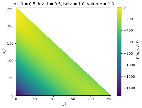
ref = lnpy.examples.load_example_lnpimasked("hsmix")
ref
<lnPi(lnz=[0.5 0.5])>
ref.xge.lnpi().plot()
<matplotlib.collections.QuadMesh at 0x7febe8ee17f0>
# function to tag 'LD' and 'HD' phases
def tag_phases2(x):
    if len(x) > 2:
        msg = "bad tag function"
        raise ValueError(msg)
    argmax0 = np.array([xx.local_argmax()[0] for xx in x])
    return np.where(argmax0 <= x[0].shape[0] / 2, 0, 1)


phase_creator = lnpy.PhaseCreator(
    nmax=2, nmax_peak=4, ref=ref, tag_phases=tag_phases2, merge_kws={"efac": 0.8}
)
build_phases = phase_creator.build_phases_mu([None, 0.0])

c = lnpy.lnPiCollection.from_builder(
    np.linspace(-5, 5, 50), build_phases, unstack=False
)
c
<class lnPiCollection>
lnz_0      lnz_1  phase
-5.000000  0.0    0                      [-5.0, 0.0]
-4.795918  0.0    0        [-4.795918367346939, 0.0]
-4.591837  0.0    0        [-4.591836734693878, 0.0]
-4.387755  0.0    0        [-4.387755102040816, 0.0]
-4.183673  0.0    0        [-4.183673469387755, 0.0]
                                     ...
 4.183673  0.0    1         [4.183673469387756, 0.0]
 4.387755  0.0    1         [4.387755102040817, 0.0]
 4.591837  0.0    1         [4.591836734693878, 0.0]
 4.795918  0.0    1         [4.795918367346939, 0.0]
 5.000000  0.0    1                       [5.0, 0.0]
Length: 65, dtype: object
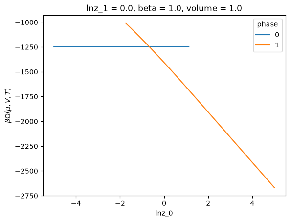
Note that here we have used the unstack=False option. This means that the results from lnpy.lnpiseries.lnPiCollection.xge will not be unstacked. For example:
c.xge.betaOmega()
<xarray.DataArray 'betaOmega' (sample: 65)> Size: 520B
array([-1246.12388491, -1246.12448998, -1246.12523222, -1246.12614278,
       -1246.12725991, -1246.1286306 , -1246.13031256, -1246.13237676,
       -1246.13491046, -1246.13802107, -1246.14184087, -1246.14653294,
       -1246.15229859, -1246.1593867 , -1246.16810551, -1246.1788377 ,
       -1246.19205972, -1010.9087438 , -1246.20836701, -1054.37219518,
       -1246.22850704, -1098.99423283, -1246.25342379, -1144.4775693 ,
       -1246.28431829, -1190.70729484, -1246.32273372, -1237.62335537,
       -1246.37067871, -1285.1875377 , -1246.43081409, -1333.37342804,
       -1246.50675309, -1382.15798324, -1246.60358765, -1431.51759825,
       -1246.72896095, -1481.42620374, -1246.89609727, -1531.84252007,
       -1247.1319439 , -1582.68976406, -1247.47204378, -1633.86017062,
       -1247.86446355, -1685.24884688, -1736.77785101, -1788.39701972,
       -1840.07559237, -1891.79461328, -1943.54206924, -1995.3100774 ,
       -2047.093286  , -2098.88794914, -2150.69137525, -2202.50158717,
       -2254.3171055 , -2306.13680626, -2357.95982463, -2409.78548824,
       -2461.61326981, -2513.44275296, -2565.27360693, -2617.10556771,
       -2668.9384238 ])
Coordinates:
  * sample   (sample) object 520B MultiIndex
  * lnz_0    (sample) float64 520B -5.0 -4.796 -4.592 -4.388 ... 4.592 4.796 5.0
  * lnz_1    (sample) float64 520B 0.0 0.0 0.0 0.0 0.0 ... 0.0 0.0 0.0 0.0 0.0
  * phase    (sample) int64 520B 0 0 0 0 0 0 0 0 0 0 0 ... 1 1 1 1 1 1 1 1 1 1 1
    beta     float64 8B 1.0
    volume   float64 8B 1.0
Attributes:
    dims_n:         ['n_0', 'n_1']
    dims_lnz:       ['lnz_0', 'lnz_1']
    dims_comp:      ['component']
    dims_state:     ['lnz_0', 'lnz_1', 'beta', 'volume']
    dims_rec:       ['sample']
    standard_name:  grand_potential
long_name: $\beta \Omega(\mu,V,T)$To ‘unstack’ from ‘sample’ dimension to ‘lnz_0’, ‘lnz_1’, etc, you can call unstack directly:
c.xge.betaOmega().unstack()
<xarray.DataArray 'betaOmega' (lnz_0: 50, lnz_1: 1, phase: 2)> Size: 800B
array([[[-1246.12388491,            nan]],

       [[-1246.12448998,            nan]],

       [[-1246.12523222,            nan]],

       [[-1246.12614278,            nan]],

       [[-1246.12725991,            nan]],

       [[-1246.1286306 ,            nan]],

       [[-1246.13031256,            nan]],

       [[-1246.13237676,            nan]],

       [[-1246.13491046,            nan]],

       [[-1246.13802107,            nan]],

...

       [[           nan, -2202.50158717]],

       [[           nan, -2254.3171055 ]],

       [[           nan, -2306.13680626]],

       [[           nan, -2357.95982463]],

       [[           nan, -2409.78548824]],

       [[           nan, -2461.61326981]],

       [[           nan, -2513.44275296]],

       [[           nan, -2565.27360693]],

       [[           nan, -2617.10556771]],

       [[           nan, -2668.9384238 ]]])
Coordinates:
  * lnz_0    (lnz_0) float64 400B -5.0 -4.796 -4.592 -4.388 ... 4.592 4.796 5.0
  * lnz_1    (lnz_1) float64 8B 0.0
  * phase    (phase) int64 16B 0 1
    beta     float64 8B 1.0
    volume   float64 8B 1.0
Attributes:
    dims_n:         ['n_0', 'n_1']
    dims_lnz:       ['lnz_0', 'lnz_1']
    dims_comp:      ['component']
    dims_state:     ['lnz_0', 'lnz_1', 'beta', 'volume']
    dims_rec:       ['sample']
    standard_name:  grand_potential
long_name: $\beta \Omega(\mu,V,T)$c.xge.betaOmega().unstack().plot(hue="phase")
[<matplotlib.lines.Line2D at 0x7febe8fb5590>,
 <matplotlib.lines.Line2D at 0x7febe8fb56d0>]
# spinodal along line of constant lnz_2

_ = c.spinodal(phase_ids=[0, 1], build_phases=build_phases, efac=1.0, inplace=True)
_ = c.binodal(phase_ids=[0, 1], build_phases=build_phases, inplace=True)
# create table for spinodal/binodal

t_spin = c.spinodal.access.xge.table(["molfrac"], ref=ref)
t_bino = c.binodal.access.xge.table(["molfrac"], ref=ref)
t_spin
<xarray.Dataset> Size: 368B
Dimensions:        (sample: 4, component: 2)
Coordinates:
  * sample         (sample) object 32B MultiIndex
  * spinodal       (sample) int64 32B 0 0 1 1
  * lnz_0          (sample) float64 32B 1.202 1.202 -1.806 -1.806
  * lnz_1          (sample) float64 32B 0.0 0.0 0.0 0.0
  * phase          (sample) int64 32B 0 1 0 1
    beta           float64 8B 1.0
    volume         float64 8B 1.0
Dimensions without coordinates: component
Data variables:
    edge_distance  (sample) float64 32B 31.11 1.0 31.11 29.7
    molfrac        (sample, component) float64 64B 0.01297 0.987 ... 0.02102
    nvec           (sample, component) float64 64B 2.715 206.5 ... 206.7 4.438
    betapV         (sample) float64 32B 1.248e+03 1.705e+03 1.246e+03 996.1
Attributes:
    dims_n:      ['n_0', 'n_1']
    dims_lnz:    ['lnz_0', 'lnz_1']
    dims_comp:   ['component']
    dims_state:  ['lnz_0', 'lnz_1', 'beta', 'volume']
    dims_rec:    ['sample']
long_name: distance from upper edget_spin.reset_index("sample").to_dataframe().query(
"component==0 and spinodal==phase"
).dropna()
| spinodal | lnz_0 | lnz_1 | phase | beta | volume | edge_distance | molfrac | nvec | betapV | ||
|---|---|---|---|---|---|---|---|---|---|---|---|
| sample | component | ||||||||||
| 0 | 0 | 0 | 1.201575 | 0.0 | 0 | 1.0 | 1.0 | 31.112698 | 0.012974 | 2.714673 | 1248.009992 |
| 3 | 0 | 1 | -1.805724 | 0.0 | 1 | 1.0 | 1.0 | 29.698485 | 0.978978 | 206.675356 | 996.095608 |
doing this for multiple values of fixed lnz_1:
from joblib import Parallel, delayed

from lnpy.stability import SpinodalError


def get_bin_spin1(lnz2, phase_creator, from_builder, from_builder_kws=None):
    # reload stability here to make sure accessor available (also make sure black keeps this here.)

    build_phases = phase_creator.build_phases_mu([None, lnz2])
    lnzs = np.linspace(-8, 8, 20)
    if from_builder_kws is None:
        from_builder_kws = {}
    c = from_builder(lnzs, build_phases, **from_builder_kws)

    try:
        c.spinodal(2, build_phases, inplace=True, unstack=False)
    except SpinodalError:
        return None, None

    c.binodal(2, build_phases, inplace=True, unstack=False)
    t_spin = c.spinodal.access.xge.table(["molfrac"], ref=ref)
    t_bino = c.binodal.access.xge.table(["molfrac"], ref=ref)
    return t_spin, t_bino
out1 = Parallel(n_jobs=-1)(
    delayed(get_bin_spin1)(lnz2, phase_creator, lnpy.lnPiCollection.from_builder)
    for lnz2 in np.arange(-5, 5, 0.5)
)
spin1 = xr.concat([s for s, b in out1 if s is not None], "sample")
bino1 = xr.concat([b for s, b in out1 if b is not None], "sample")
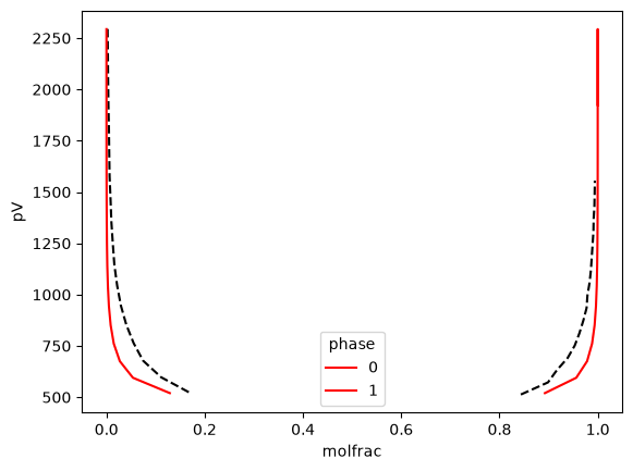
def plot_frame(df, **kws) -> None:
    (
        df
        .reset_index()
        .set_index(["molfrac", "phase"])
        .assign(pV=lambda x: x["betapV"] / x["beta"])["pV"]
        .to_xarray()
        .plot(hue="phase", **kws)
    )


plot_frame(
    spin1
    .reset_index("sample")
    .to_dataframe()
    .query("component==0 and spinodal==phase")
    .dropna(),
    ls="--",
    color="k",
)
plot_frame(
    bino1.reset_index("sample").to_dataframe().query("component==0").dropna(), color="r"
)