Outlier Detection: Recursive

Imports

#Python modules for numerics and scientific computing
import numpy as np
import pandas as pd
import scipy as sp
import math

#scikit-learn
import sklearn.preprocessing as skpp
import sklearn.decomposition as skdecomp

#Matplotlib
%matplotlib inline
import matplotlib
import matplotlib.pyplot as plt
import matplotlib.colors as mcolors
import matplotlib.lines as mlines
import matplotlib.patches as mpatches

import mab_utils
import plot_utils as plu
#import tqdm

import interlab as inl
import pickle

Load data from processing notebook

jeffries = r'Symmetric Kullback-Liebler'

with open('mAb_interlab_project.sav','rb') as f:
    mab_project = pickle.load(f)

with open('mab_analysis_accessories.sav','rb') as f:
    (windowed_shape,jeffries,full_indices,split_point,
     ssi_contours,interp_map) = pickle.load(f)

metadata_table = pd.read_hdf('metadata_table_raw.h5',key='NMR_2D_raw',mode='r')

Calculate probability scores and find outliers

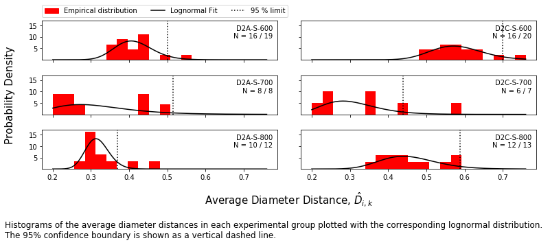
The matrix of pairwise distances is collapsed into the vector of average distances by taking the average distance of each spectrum from each other. The population of average distances in each group is fit to a distribution (here, lognormal).

mab_project.fit_zscores()

Probability scores are calculated for each measurement within each group and spectra outside the 95 % confidence boundary are identified as outliers.

mab_project.find_outliers(recursive=True,
                          support_fraction=0.85,
                          final_screen=True
                         )

plot_range = ['D2A-S-600',
              'D2A-S-700',
              'D2A-S-800',
              'D2C-S-600',
              'D2C-S-700',
              'D2C-S-800',
             ]

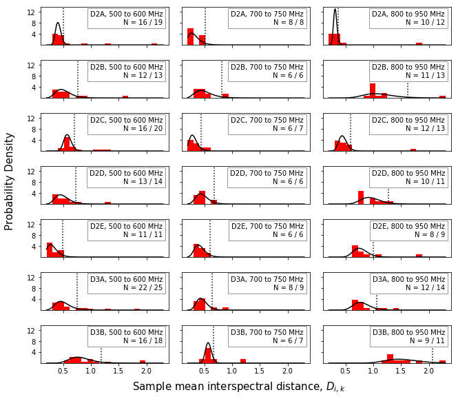
f = mab_project.plot_histograms(jeffries,plot_range=plot_range,#['D2A-S-600','D2C-S-600'],
                                numcols=2)


empirical_red_patch = mpatches.Patch(color='red', label='Empirical distribution')
lognormal_line = mlines.Line2D([],[],color='k',label='Lognormal Fit')
confidence_limit = mlines.Line2D([],[],color='k',ls=':',label='95 % limit')
l = f.axes[0].legend(handles=[empirical_red_patch,lognormal_line,confidence_limit],
                     ncol=3,loc=(0.0,1.1))

caption_text = ('Histograms of the average diameter distances in each experimental group ' +
                'plotted with the corresponding lognormal distribution. \nThe 95% ' +
                'confidence boundary is shown as a vertical dashed line. '
               )

width,height = f.get_size_inches()

t = f.text(0,-0.25/height,caption_text,size=12,va='top')

Save outlier information to metadata table

Outlier data from the interlab study is saved to our metadata table.

mab_utils.save_outlier_data(metadata_table,mab_project,full_indices,
                                        split_point,metric=jeffries)
metadata_table.head(5)

	INDEX	DIR_NAME	CODE	TITLE	ExpType	ExpCode	File	ExptScore	Zscore	Outlier
0	1	8822	8822-010	D2C-S-U-900-8822-010-37C	800	D2C-S	./release3/new_ext/001-D2C-S-U-900-8822-010-37...	0	0.851621	False
1	2	7425	7425-010	D2A-S-U-900-7425-010-37C	800	D2A-S	./release3/new_ext/002-D2A-S-U-900-7425-010-37...	0	0.810390	False
2	3	7425	7425-012	D2C-S-U-900-7425-012-37C	800	D2C-S	./release3/new_ext/003-D2C-S-U-900-7425-012-37...	0	0.529562	False
3	4	7425	7425-015	D3A-F-U-900-7425-015-37C	800	D3A-F	./release3/new_ext/004-D3A-F-U-900-7425-015-37...	0	0.426977	False
4	5	8495	8495-010	D2A-S-U-900-8495-010-37C	800	D2A-S	./release3/new_ext/005-D2A-S-U-900-8495-010-37...	0	11.433257	False

Outlier spectra

plot_dict = dict(xlabel='$^1$H shift (ppm)',
                 ylabel='$^{13}$C shift (ppm)',
                 plot_corners = [1.9,-0.9,30.5,9],
                 shape=windowed_shape,
                 window=False,
                 sharex=True,sharey=True,
                 plotsize=(3,2),gridspec_kw=dict(hspace=0.05,wspace=0.05))

contour_colors_mappable = matplotlib.cm.ScalarMappable(
    cmap=mab_utils.seismic_with_alpha.reversed())

contour_colormap = contour_colors_mappable.get_cmap()
contours_rescale = np.interp(ssi_contours,*interp_map)

contour_colors = contour_colormap(contours_rescale)

False-positive outliers

match_code = np.array([code.startswith('D') for code in metadata_table.ExpCode.values])
match_expert =  np.array([score==0 for score in metadata_table.ExptScore.values])
match_algori = np.array(metadata_table.Outlier)
match_outlier = np.logical_and(match_expert,match_algori)
#match_outlier =  np.logical_or(np.array(metadata_table.Outlier),np.array(metadata_table.LabOutlier))
match = np.logical_and(match_outlier,match_code)
bbox = dict(facecolor='w')

exps = metadata_table.iloc[match]
fig,axes = mab_utils.plot_the_nmr(exps,ncols=4,
                                  levels=ssi_contours,
                                  color=contour_colors,
                                  **plot_dict)
ax = axes.flatten()[0]
ax.invert_xaxis()
ax.invert_yaxis()
for score,ax in zip(metadata_table.ExptScore.values[match],axes.flatten()):
    ax.text(0.95,0.95,str(score),ha='right',va='top',transform=ax.transAxes,bbox=bbox)

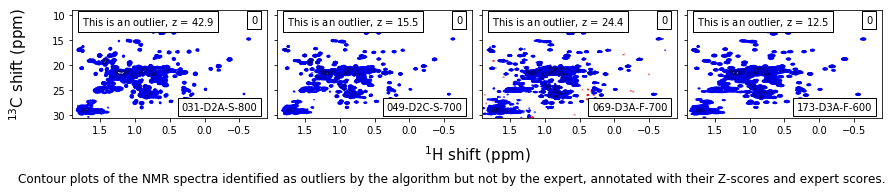
caption_text = ('Contour plots of the NMR spectra identified as outliers by the algorithm ' +
                'but not by the expert, annotated with their Z-scores and expert scores.'
               )
width,height = fig.get_size_inches()

t = fig.text(0,-0.25/height,caption_text,size=12,va='top')

/home/local/NIST/dsheen/.conda/envs/default_outside/lib/python3.7/site-packages/matplotlib/contour.py:1000: UserWarning: The following kwargs were not used by contour: 'aspect'
  s)

Expert level-2 outliers

match_code = np.array([code.startswith('D') for code in metadata_table.ExpCode.values])
match_outlier =  np.array([score>1 for score in metadata_table.ExptScore.values])
#match_outlier =  np.logical_or(np.array(metadata_table.Outlier),np.array(metadata_table.LabOutlier))
match = np.logical_and(match_outlier,match_code)
bbox = dict(facecolor='w')

exps = metadata_table.iloc[match]
fig,axes = mab_utils.plot_the_nmr(exps,ncols=4,
                                  levels=ssi_contours,
                                  color=contour_colors,
                                  **plot_dict)
ax = axes.flatten()[0]
ax.invert_xaxis()
ax.invert_yaxis()
for score,ax in zip(metadata_table.ExptScore.values[match],axes.flatten()):
    ax.text(0.95,0.95,str(score),ha='right',va='top',transform=ax.transAxes,bbox=bbox)

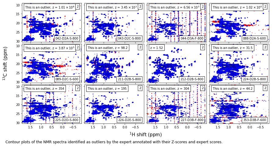
caption_text = ('Contour plots of the NMR spectra identified as outliers by the expert ' +
                'annotated with their Z-scores and expert scores.'
               )
width,height = fig.get_size_inches()

t = fig.text(0,-0.25/height,caption_text,size=12,va='top')

Expert level-1 outliers

match_code = np.array([code.startswith('D') for code in metadata_table.ExpCode.values])
match_outlier =  np.array([score==1 for score in metadata_table.ExptScore.values])
#match_outlier =  np.logical_or(np.array(metadata_table.Outlier),np.array(metadata_table.LabOutlier))
match = np.logical_and(match_outlier,match_code)
bbox = dict(facecolor='w')

exps = metadata_table.iloc[match]
fig,axes = mab_utils.plot_the_nmr(exps,ncols=4,
                                  levels=ssi_contours,
                                  color=contour_colors,
                                  **plot_dict)
ax = axes.flatten()[0]
ax.invert_xaxis()
ax.invert_yaxis()
for score,ax in zip(metadata_table.ExptScore.values[match],axes.flatten()):
    ax.text(0.95,0.95,str(score),ha='right',va='top',transform=ax.transAxes,bbox=bbox)

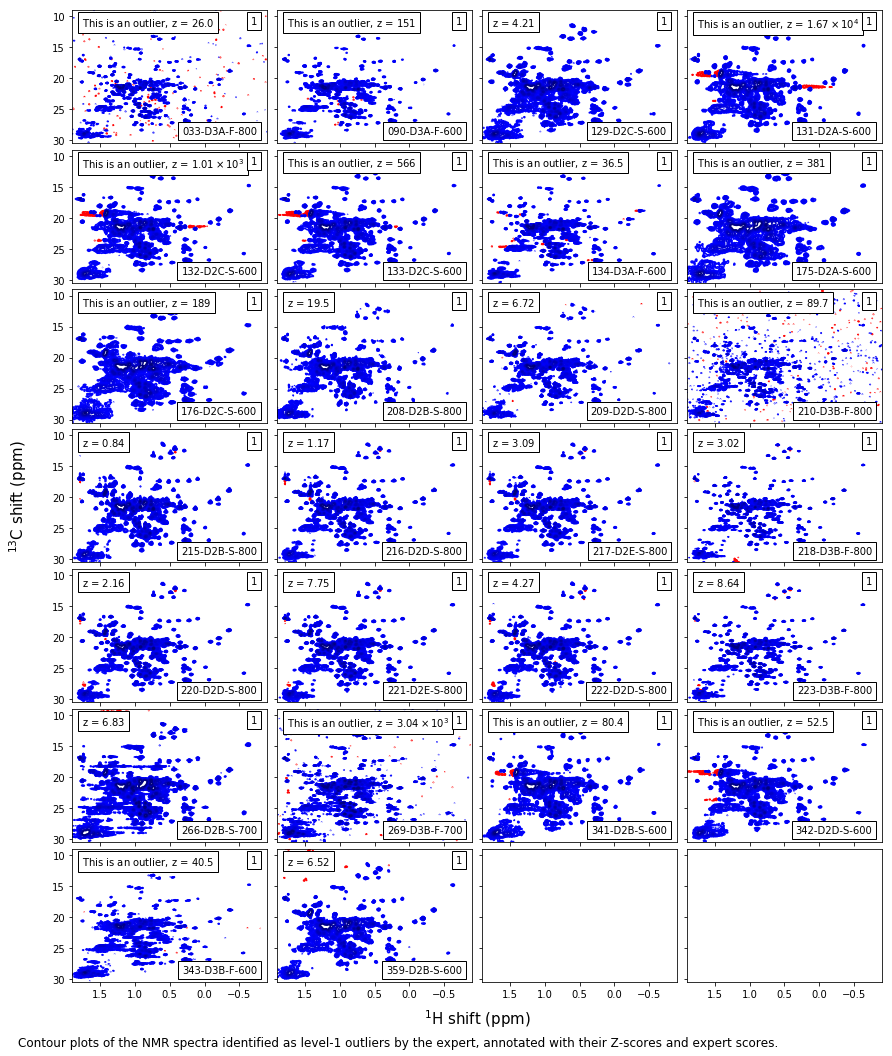
caption_text = ('Contour plots of the NMR spectra identified as level-1 outliers by ' +
                'the expert, annotated with their Z-scores and expert scores.'
               )

width,height = fig.get_size_inches()

t = fig.text(0,-0.25/height,caption_text,size=12,va='top')

metadata_table.to_csv('metadata_table_recursive.csv',sep='\t')

keys_no_e = []
for key in ['600','700','800']:
    keys_no_e += [k for k in mab_project.Labels.keys()
                  if k.startswith('D') and k.endswith(key)]

bbox_props = dict(edgecolor='0.6',facecolor='w')
f = mab_project.plot_histograms(jeffries,numcols=3,plot_range=keys_no_e)
size = f.get_size_inches()
vert_size = size[1]#*1.75
horz_size = size[0]/1.75
f.set_size_inches((horz_size,vert_size,))
for a in f.axes:
    t = a.texts[0]
    t_str = t.get_text()
    type_string = '-S-'
    if '-F-' in t_str:type_string = '-F-'
    if '600' in t_str:t_str = t_str.replace(type_string+'600',', 500 to 600 MHz')
    if '700' in t_str:t_str = t_str.replace(type_string+'700',', 700 to 750 MHz')
    if '800' in t_str:t_str = t_str.replace(type_string+'800',', 800 to 950 MHz')
    t.set_text(t_str)
    t.set_bbox(bbox_props)
    t.set_position((0.95,0.9))
f.texts[1].set_text('Sample mean interspectral distance, $D_{i,k}$')
f.subplots_adjust(left=0.08,bottom=0.08,wspace=0.0)

means = []
threshes = []
names = []
for x in mab_project:
    if x.name in keys_no_e:
        pop = x[jeffries].population
        params = pop.params
        dist = pop.distribution
        mean = dist.mean(*params)
        thresh = dist.ppf(0.9495,*params)

        name = x.name



        type_string = '-S-'
        if '-F-' in name:type_string = '-F-'
        if '600' in name:name = name.replace(type_string+'600',', low')
        if '700' in name:name = name.replace(type_string+'700',', med')
        if '800' in name:name = name.replace(type_string+'800',', high')

        print('{}: {:5.3f} {:5.3f}'.format(name,mean,thresh))

        means += [mean]
        threshes += [thresh]
        names += [name]

        #print(,params)

D2A, low: 0.414 0.500
D2A, med: 0.319 0.515
D2A, high: 0.317 0.370
D2B, low: 0.514 0.770
D2B, med: 0.507 0.814
D2B, high: 1.121 1.622
D2C, low: 0.583 0.700
D2C, med: 0.307 0.440
D2C, high: 0.457 0.588
D2D, low: 0.494 0.729
D2D, med: 0.468 0.676
D2D, high: 0.962 1.270
D2E, low: 0.311 0.491
D2E, med: 0.424 0.599
D2E, high: 0.775 1.003
D3A, low: 0.504 0.756
D3A, med: 0.462 0.638
D3A, high: 0.800 1.064
D3B, low: 0.825 1.183
D3B, med: 0.577 0.669
D3B, high: 1.537 2.065

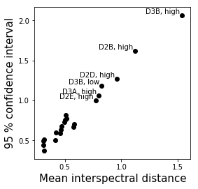
fig,ax = plt.subplots(figsize=(4,4))

ax.scatter(means,threshes,color='k')
ax.set_xlabel('Mean interspectral distance',size=15)
ax.set_ylabel('95 % confidence interval',size=15)
ax.set_yticks([0.5,1,1.5,2])
ax.set_xticks([0.5,1,1.5])
for n,m,t in zip(names,means,threshes):
    if t > 1:    ax.text(m-0.02,t,n,ha='right',va='bottom')