Outlier Detection: Refit to single population

Imports

#Python modules for numerics and scientific computing
import numpy as np
import pandas as pd
import scipy as sp
import math

#scikit-learn
import sklearn.preprocessing as skpp
import sklearn.decomposition as skdecomp

#Matplotlib
%matplotlib inline
import matplotlib
import matplotlib.pyplot as plt
import matplotlib.colors as mcolors
import matplotlib.lines as mlines
import matplotlib.patches as mpatches

import mab_utils
import plot_utils as plu
#import tqdm

import interlab as inl
import interlab.utilities
import pickle

Load data from processing notebook

jeffries = r'Symmetric Kullback-Liebler'

with open('mAb_interlab_project.sav','rb') as f:
    mab_project = pickle.load(f)

with open('mab_analysis_accessories.sav','rb') as f:
    (windowed_shape,jeffries,full_indices,split_point,
     ssi_contours,interp_map) = pickle.load(f)

metadata_table = pd.read_hdf('metadata_table_raw.h5',key='NMR_2D_raw',mode='r')

Calculate probability scores and find outliers

The matrix of pairwise distances is collapsed into the vector of average distances by taking the average distance of each spectrum from each other. The population of average distances in each group is fit to a distribution (here, lognormal).

mab_project.fit_zscores()

Probability scores are calculated for each measurement within each group and spectra outside the 95 % confidence boundary are identified as outliers.

mab_project.find_outliers(recursive=False,support_fraction=0.6)

mab_utils.save_outlier_data(metadata_table,mab_project,full_indices,
                                        split_point,metric=jeffries)

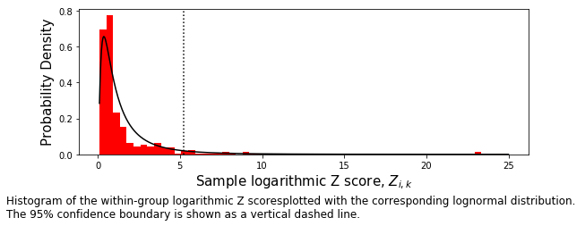
The entire set of Z-scores is then used as a single population and a new distribution is fit.

normalized_scores = metadata_table.Zscore.values

new_pop = inl.utilities.Population('All spectra normalized',
                                  distribution=sp.stats.lognorm,
                                   values=normalized_scores
                                  )

new_pop.fit_zscores()
new_pop.find_outliers()
f,ax = plt.subplots(figsize=(9,3))
new_pop.histogram(ax,num_bins=60)
t=ax.set_xlabel(r"Sample logarithmic Z score, $Z_{i,k}$",size=15)
t=ax.set_ylabel("Probability Density",size=15)

caption_text = ('Histogram of the within-group logarithmic Z scores' +
                'plotted with the corresponding lognormal distribution. \nThe 95% ' +
                'confidence boundary is shown as a vertical dashed line. '
               )

width,height = f.get_size_inches()

t = f.text(0,-0.25/height,caption_text,size=12,va='top')

fig,ax = plt.subplots(figsize=(19,3)) new_pop.plot_zscores(ax,rotation='vertical') t=ax.set_ylabel("Sample logarithmic\nZ score, $Z_{i,k}$",size=15) ax.axhline(5.1,color='k',ls=':') for tx in ax.texts: tx.set_visible(False)plot_range = ['D2A-S-600', 'D2A-S-700', 'D2A-S-800', 'D2C-S-600', 'D2C-S-700', 'D2C-S-800', ] f = mab_project.plot_histograms(jeffries,plot_range=plot_range,#['D2A-S-600','D2C-S-600'], numcols=2) empirical_red_patch = mpatches.Patch(color='red', label='Empirical distribution') lognormal_line = mlines.Line2D([],[],color='k',label='Lognormal Fit') confidence_limit = mlines.Line2D([],[],color='k',ls=':',label='95 % limit') l = f.axes[0].legend(handles=[empirical_red_patch,lognormal_line,confidence_limit], ncol=3,loc=(0.0,1.1)) caption_text = ('Histograms of the average diameter distances in each experimental group ' + 'plotted with the corresponding lognormal distribution. \nThe 95% ' + 'confidence boundary is shown as a vertical dashed line. ' ) width,height = f.get_size_inches() t = f.text(0,-0.25/height,caption_text,size=12,va='top')

Save outlier information to metadata table

Outlier data from the interlab study is saved to our metadata table.

metadata_table.Zscore = new_pop.zscores
metadata_table.Outlier = ~new_pop.outlier_mask
metadata_table.head(5)

	INDEX	DIR_NAME	CODE	TITLE	ExpType	ExpCode	File	ExptScore	Zscore	Outlier
0	1	8822	8822-010	D2C-S-U-900-8822-010-37C	800	D2C-S	./release3/new_ext/001-D2C-S-U-900-8822-010-37...	0	0.715926	False
1	2	7425	7425-010	D2A-S-U-900-7425-010-37C	800	D2A-S	./release3/new_ext/002-D2A-S-U-900-7425-010-37...	0	0.670746	False
2	3	7425	7425-012	D2C-S-U-900-7425-012-37C	800	D2C-S	./release3/new_ext/003-D2C-S-U-900-7425-012-37...	0	0.586484	False
3	4	7425	7425-015	D3A-F-U-900-7425-015-37C	800	D3A-F	./release3/new_ext/004-D3A-F-U-900-7425-015-37...	0	0.507501	False
4	5	8495	8495-010	D2A-S-U-900-8495-010-37C	800	D2A-S	./release3/new_ext/005-D2A-S-U-900-8495-010-37...	0	1.115246	False

Outlier spectra

plot_dict = dict(xlabel='$^1$H shift (ppm)',
                 ylabel='$^{13}$C shift (ppm)',
                 plot_corners = [1.9,-0.9,30.5,9],
                 shape=windowed_shape,
                 window=False,
                 sharex=True,sharey=True,
                 plotsize=(3,2),gridspec_kw=dict(hspace=0.05,wspace=0.05))

contour_colors_mappable = matplotlib.cm.ScalarMappable(
    cmap=mab_utils.seismic_with_alpha.reversed())

contour_colormap = contour_colors_mappable.get_cmap()
contours_rescale = np.interp(ssi_contours,*interp_map)

contour_colors = contour_colormap(contours_rescale)

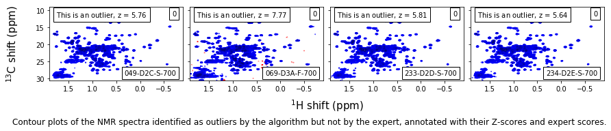
False-positive outliers

match_code = np.array([code.startswith('D') for code in metadata_table.ExpCode.values])
match_expert =  np.array([score==0 for score in metadata_table.ExptScore.values])
match_algori = np.array(metadata_table.Outlier)
match_outlier = np.logical_and(match_expert,match_algori)
#match_outlier =  np.logical_or(np.array(metadata_table.Outlier),np.array(metadata_table.LabOutlier))
match = np.logical_and(match_outlier,match_code)
bbox = dict(facecolor='w')

exps = metadata_table.iloc[match]
fig,axes = mab_utils.plot_the_nmr(exps,ncols=4,
                                  levels=ssi_contours,
                                  color=contour_colors,
                                  **plot_dict)
ax = axes.flatten()[0]
ax.invert_xaxis()
ax.invert_yaxis()
for score,ax in zip(metadata_table.ExptScore.values[match],axes.flatten()):
    ax.text(0.95,0.95,str(score),ha='right',va='top',transform=ax.transAxes,bbox=bbox)

caption_text = ('Contour plots of the NMR spectra identified as outliers by the algorithm ' +
                'but not by the expert, annotated with their Z-scores and expert scores.'
               )
width,height = fig.get_size_inches()

t = fig.text(0,-0.25/height,caption_text,size=12,va='top')

/home/local/NIST/dsheen/.conda/envs/default_outside/lib/python3.7/site-packages/matplotlib/contour.py:1000: UserWarning: The following kwargs were not used by contour: 'aspect'
  s)

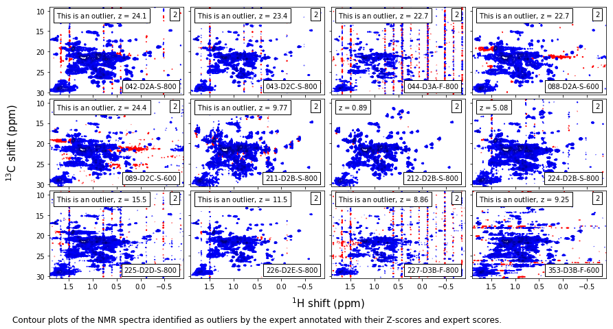
Expert level-2 outliers

match_code = np.array([code.startswith('D') for code in metadata_table.ExpCode.values])
match_outlier =  np.array([score>1 for score in metadata_table.ExptScore.values])
#match_outlier =  np.logical_or(np.array(metadata_table.Outlier),np.array(metadata_table.LabOutlier))
match = np.logical_and(match_outlier,match_code)
bbox = dict(facecolor='w')

exps = metadata_table.iloc[match]
fig,axes = mab_utils.plot_the_nmr(exps,ncols=4,
                                  levels=ssi_contours,
                                  color=contour_colors,
                                  **plot_dict)
ax = axes.flatten()[0]
ax.invert_xaxis()
ax.invert_yaxis()
for score,ax in zip(metadata_table.ExptScore.values[match],axes.flatten()):
    ax.text(0.95,0.95,str(score),ha='right',va='top',transform=ax.transAxes,bbox=bbox)

caption_text = ('Contour plots of the NMR spectra identified as outliers by the expert ' +
                'annotated with their Z-scores and expert scores.'
               )
width,height = fig.get_size_inches()

t = fig.text(0,-0.25/height,caption_text,size=12,va='top')

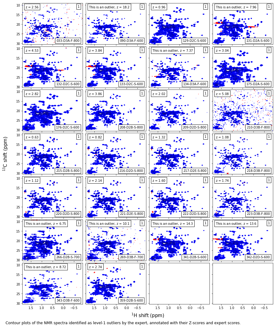
Expert level-1 outliers

match_code = np.array([code.startswith('D') for code in metadata_table.ExpCode.values])
match_outlier =  np.array([score==1 for score in metadata_table.ExptScore.values])
#match_outlier =  np.logical_or(np.array(metadata_table.Outlier),np.array(metadata_table.LabOutlier))
match = np.logical_and(match_outlier,match_code)
bbox = dict(facecolor='w')

exps = metadata_table.iloc[match]
fig,axes = mab_utils.plot_the_nmr(exps,ncols=4,
                                  levels=ssi_contours,
                                  color=contour_colors,
                                  **plot_dict)
ax = axes.flatten()[0]
ax.invert_xaxis()
ax.invert_yaxis()
for score,ax in zip(metadata_table.ExptScore.values[match],axes.flatten()):
    ax.text(0.95,0.95,str(score),ha='right',va='top',transform=ax.transAxes,bbox=bbox)

caption_text = ('Contour plots of the NMR spectra identified as level-1 outliers by ' +
                'the expert, annotated with their Z-scores and expert scores.'
               )

width,height = fig.get_size_inches()

t = fig.text(0,-0.25/height,caption_text,size=12,va='top')

metadata_table.to_csv('metadata_table_single-pop.csv',sep='\t')