Example interlaboratory study
Imports
Import the mumpce interface and the interface to interlab.
[1]:
import interlab as inl
Import Numerical Python and Pandas
[2]:
import pandas as pd
import numpy as np
import matplotlib.pyplot as plt
Creating a Project
Reading project metadata
interlab is agnostic to the way that your data is arranged. All that’s required is that you have the experimental measurements divided logically into groups, where each group represents all the measurements of one sample. The exact way you do this is up to you; this example shows how to do create a Project using Pandas and an Excel workbook.
We’ve decided to remove some of the NMR data in the region of the water signal, so let’s define the range that we’ll actually use.
[3]:
range_to_use = list(range(959)) + list(range(1058,1860))
Read the Excel workbook that contains the project data. We’re using Pandas to read all the sheets of this workbook. This will result in a dictionary of Pandas DataFrame objects that we will have to parse.
[4]:
df_dict = pd.read_excel('syn_data.xlsx',sheet_name=None)
Each sheet in the workbook corresponds to the NMR spectra from one particular sample. The name of each sheet is the name of the sample, which are then the keys of our df_dict. We’ll use these keys as the keys for the various dictionaries we make before we create the Project.
[5]:
Spectrum_names = [key for key,df in df_dict.items()]
print(Spectrum_names)
['S1a', 'S1b', 'S1c', 'S1d', 'S1e', 'S1f', 'S2', 'S3', 'S4', 'S5', 'S6']
The sheets are arranged such that each row corresponds to an NMR bin and each column represents the NMR measurements from one facility. We’ll extract the index values as the X data for our spectra and the column values as our list of facility labels. The X data have to be the same across all measurements, so we don’t save this as a dictionary. However, the facility labels might be different, because not every facility may have values for every experiment. This needs to be a dictionary with one element for every experiment.
[6]:
Labels_dict = {}

for key,df in df_dict.items():
    peakPPM_full = df.index.values[range_to_use]
    Labels = df.columns.values
    Labels_dict[key] = df.columns.values

print(Labels)
print(peakPPM_full)
['0115' '0122' '0258' '0333' '0711' '0714' '2861' '7042' '8865' '9541']
[9.9975 9.9925 9.9875 ... 0.2125 0.2075 0.2025]
Here, we define which metrics we’ll be using for the interlab analysis.
[7]:
jeffries = r'Symmetric Kullback-Liebler'
jensen = r'Jensen-Shannon'
hellinger = r'Hellinger'
mahalanobis = r'Mahalanobis'
nmr_distance_metrics = [dict(metric=mahalanobis,function='mahalanobis'),
                        dict(metric=hellinger,function=inl.metrics.hellinger_hyp),
                        dict(metric=jeffries,function=inl.metrics.jeffries),
                        dict(metric=jensen,function=inl.metrics.jensen_hyp)
                       ]
Reading project data
Now that the metadata have all been read, we will actually read the data and create the data dictionaries. We extract the raw data for each experiment group directly from the dataframe, after we remove the water-signal data that we didn’t want. This data goes into rawdata_dict. We use fix_spectrum to remove negative and zero values, then we sum-normalize the spectra. This goes into data_dict, which will actually be used for the interlab analysis.
[8]:
rawdata_dict = {}
data_dict = {}

for key,df in df_dict.items():
    raw_values = df.values[range_to_use].T
    rawdata_dict[key] = raw_values

    normalized_values = inl.fix_spectrum(raw_values)
    data_dict[key] = (normalized_values.T/normalized_values.sum(axis=1)).T
Creating the Project
Now we have enough data to create the Project object. When created, the Project will read the rawdata_dict, data_dict, and Labels_dict, associating each element of these dictionaries with an ExperimentGroup object.
[9]:
synthetic_samples_project = inl.Project(x_data_list=peakPPM_full,
                                         Sample_names=Spectrum_names,
                                         Data_set_names=Labels_dict,
                                         distance_metrics=nmr_distance_metrics,
                                         data=data_dict,rawdata=rawdata_dict)
Using Projects to run interlaboratory analysis
Now that we’ve created the project, we can begin to run the interlab analysis.
Interspectral distance matrices
Interspectral covariance matrix
Since we’re using Mahalanobis distance as a metric, we need to calculate the inverse covariance matrix. As there are fewer observations than variables, we know the covariance matrix will be singular, so we need to use the singular value decomposition to calculate it.
[10]:
synthetic_samples_project.process_mahalanobis()
Distance matrices
Now we calculate the distance matrices for each group,
[11]:
synthetic_samples_project.set_distances()
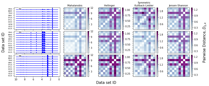
We can plot the spectral data and the distance matrices. Note that, if plot_range isn’t specified, this function will plot all of them
[12]:
f = synthetic_samples_project.plot_distance_fig(linecolor='b',cmap='BuPu',
                                                plot_range=['S2','S3','S6'])
Sample-level scores and outliers
Fit the scores to the distances, and then find the outliers.
[13]:
synthetic_samples_project.fit_zscores()
synthetic_samples_project.find_outliers()
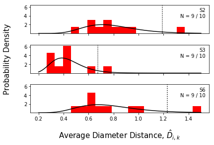
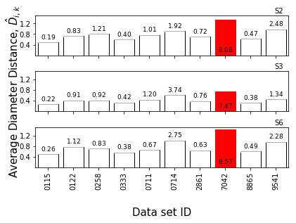
We can also plot histograms and bar charts of the average interspectral distances. These distributions are where the Z-scores come from.
Again, plot_range is optional.
[14]:
f = synthetic_samples_project.plot_histograms(jeffries,
                                              numcols=1,
                                              plot_range=['S2','S3','S6'])
f = synthetic_samples_project.plot_zscore_distances(jeffries,
                                                    numcols=1,
                                                    plot_range=['S2','S3','S6'])
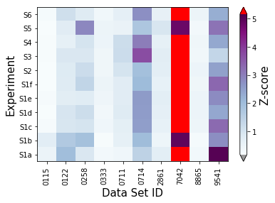
Interlaboratory statistical projection
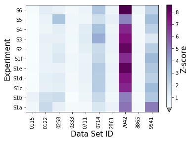
The Z-scores can then be cast as an array, which we will then use to calculate the lab-level scores and determine outliers. Note how, in this case, we are not screening outlier spectra before we perform our analysis.
[15]:
synthetic_samples_project.extract_matrices(screen_outliers=False)
synthetic_samples_project.plot_zscores_heatmap(metric=jeffries,cmap='BuPu')
synthetic_samples_project.plot_zscores_heatmap(screen_outliers=False,metric=jeffries,cmap='BuPu')
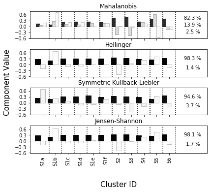
f = synthetic_samples_project.plot_zscore_loadings()
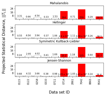
Laboratory-level scoring and outliers
Find the outliers and plot the lab-level Z-scores as well as the statistical projection
[16]:
synthetic_samples_project.find_lab_outliers(recursive=True,support_fraction=0.6)
f = synthetic_samples_project.plot_projected_zscores()
f = synthetic_samples_project.plot_zscore_outliers(jeffries)
f.axes[0].set_aspect('equal')
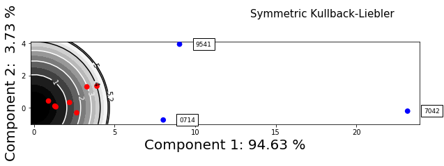
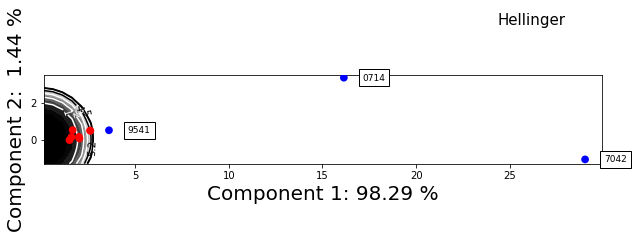
[17]:
f = synthetic_samples_project.plot_zscore_outliers(hellinger)
f.axes[0].set_aspect('equal')
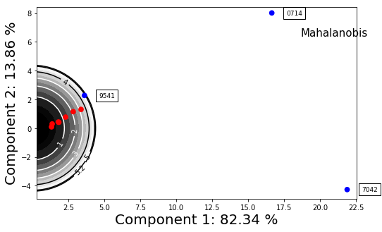
[18]:
f = synthetic_samples_project.plot_zscore_outliers(mahalanobis)
f.axes[0].set_aspect('equal')
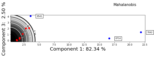
f = synthetic_samples_project.plot_zscore_outliers(mahalanobis,y_component=2)
f.axes[0].set_aspect('equal')
Accessing data within a Project
Accessing Experiment Groups
The individual ExperimentGroup objects can be accessed as if the Project were a dictionary:
[19]:
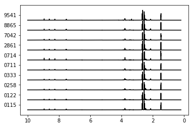
nmrdata = synthetic_samples_project['S6'].data.T
nmrdata = nmrdata/nmrdata.max(axis=0)
plt.plot(peakPPM_full,nmrdata+range(10),color='k')
plt.gca().set_yticks(np.array(range(10))+0.5)
plt.gca().set_yticklabels(Labels)
plt.gca().invert_xaxis()
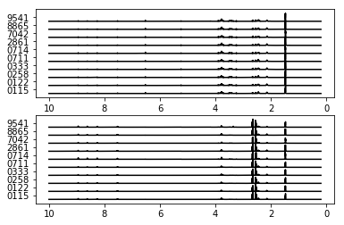
You can access multiple ExperimentGroup objects by passing a list of names.
[20]:
group_list = synthetic_samples_project[['S2','S6']]

fig,axes = plt.subplots(2,1)

for group,ax in zip(group_list,axes):
    nmrdata= group.data.T
    nmrdata = nmrdata/nmrdata.max(axis=0)
    ax.plot(peakPPM_full,nmrdata+range(10),color='k')
    ax.set_yticks(np.array(range(10))+0.5)
    ax.set_yticklabels(Labels)
    ax.invert_xaxis()
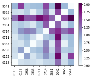
Accessing Distance Metrics
Individual DistanceMetric objects for an ExperimentGroup can be accessed by array-like indexing:
[21]:
d = synthetic_samples_project['S6',jeffries].distance_matrix
plt.imshow(d,origin='lower',cmap='BuPu')
plt.gca().set_yticks(np.array(range(10)))
plt.gca().set_yticklabels(Labels)
plt.gca().set_xticks(np.array(range(10)))
plt.gca().set_xticklabels(Labels,rotation='vertical')
plt.colorbar()
[21]:
<matplotlib.colorbar.Colorbar at 0x7fa4005ece48>
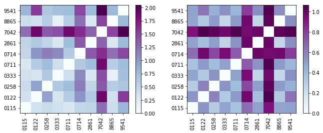
Multiple DistanceMetric objects can be accessed by passing a list.
[22]:
metric_list = synthetic_samples_project['S6',[jeffries,hellinger]]

fig,axes = plt.subplots(1,2,figsize=(11,4))

for metric,ax in zip(metric_list,axes):
    d = metric.distance_matrix
    im = ax.imshow(d,origin='lower',cmap='BuPu')
    ax.set_yticks(np.array(range(10)))
    ax.set_yticklabels(Labels)
    ax.set_xticks(np.array(range(10)))
    ax.set_xticklabels(Labels,rotation='vertical')
    fig.colorbar(im,ax=ax)
[ ]: