Appendix B: Linear State Estimation (LSE) Example Application
Introduction
Electromechanical dynamic models are widely used to study transient and small signal stability problems in power systems. States are the minimum set of variables that can determine the status of a dynamic system. A dynamic model with accurate states can faithfully reveal system responses and therefore be used to enhance system stability and reliability of a power system.
Therefore, the main objective of state estimation is to find the voltage phasors of all the bars or buses of the system. To understand the methodology, a classic observation model is described below:
Where \(\mathbf{z}\) is a vector \(\in \ \mathbb{R}^{\text{mx}1}\) containing the m measurements from all the sensing devices installed in the network, \(\mathbf{x}\mathbf{\ \in \ }\mathbb{R}^{2\text{nx}1}\mathbf{\ }\) is the state vector with the voltage phasors of the n buses of the electrical system, \(h()\) is a \(\mathbb{R}^{2n}\ \rightarrow \mathbb{R}^{m}\) function which relates the voltage phasors to the measurements. Now, if the system relies exclusively on PMU phasor measurements, the model can be expressed in linear form:
Otherwise if there are measurements such as active and reactive power (SCADA case) the function \(h\) is non-linear, and iterative methods such as Gauss-Newton must be used to reach a solution. At the end of this annex a sub-annex that shows how to obtain the measurement matrix \(H\ \mathbf{\in \ }\mathbb{R}^{\text{mx}2n}\) is explained. To estimate the optimal value of the state vector, the Weighted Least Squares (WLS) method is proposed, in accordance with this approach the following objective function is defined:
Where \(R\) is the covariance matrix of the measurements. The optimal solution that minimizes the objective function is:
Where \({\hat{\mathbf{x}}}_{\text{LS}}\) is the least square estimator we were looking for.
Some of this example is based upon work done at Washington State University [1].
Getting Started
Before the LSE examples can be run, some first-time setup is required. These instructions are the same as found in Quick Start
The Linear State Estimation Example Application uses two Matlab toolboxes that need to be downloaded:
Go to the PSERC MatPower Page and click
Download Now.Unzip the downloaded file into your Documents\MATLAB\Toolbox folder.
Add the path to MatPower to the Matlab Path using the instructions in the Matlab
pathtoolsimilar to the Matlab Path section above.PARTF requires some of the .m files in MatPower to be modified. Find the following folder: <partf install path)\Modules\MATLAB\Events\IEEEBus\IEEE cases, copy the nine ‘case##.m’ files and copy them to the matpower main folder, replacing the files that were there. The most part of the files are the same, but little modifications were made to save the reference voltages of the IEEE systems.
The LSE Application Example also includes Dynamic Events. These examples require the Matlab Power System Toolbox available from The Royal Institute of Technology in Stockholm, Sweden.
Download PSTV3, PST Data, and the Manual
You will need to register and get a password
As with the MatPower toolbox, unzip these into your Documents\MATLAB\Toolbox folder and set up the Matlab Path
Note that the Power System Toolbox is not open source software and cannot be redistributed.
Example Linear State Estimation
Creation of a stationary event case for a IEEE standard system
The MATPOWER toolbox installed during the first-time setup is used to create IEEEBusSystem test (.tst) files., With these files, the PMUs could be in any location and in any IEEE bus system that the user desires. To do that please take a look at the My Documents\PARTF\Tests\LSE\IEEEBusSystem_test_creator.m file. From there you will find the user input variables which you will be able to change:
- user_pmu_list []: The bar or the buses were the PMUs are located.
- IEEE_bus_selection: The IEEE system under test
- NoiseVariance: The noise variance of the AWNG of the magnitude and phase signals.
- The event configuration parameters:
- Start time:
- End time:
- PosSeq:
- Nominal Frequency:
- Reporting Rate:
- FSamp:
- The PMU impairment parameters:
- PMUImpairPluginINIFilePath
- FilterType:
- PmuImpairParams:
If you run this MATLAB code, you are creating a .tst file in the Test files directory. The name of the file created reflects the IEEE system selected as well also the number of PMUs associated (by default: IEEEBusSystem_case14_4pmus.tst).
If the PARTF framework is not running, start it now. Click the file browse button in the Test File control and select the newly created file in ..\tests\LSE (IEEEBusSystem_case14_4pmus.tst by default). Next click the Open button. 4 buses will be created.
To watch the results as they are computed launch the VisualizeAppLSE.vi by clicking on the Visualization button in the top right of the PARTF panel. VisualizeAllLSE should be pre-checked so click the Run Apps button to launch the visualization app. Visualization apps give the user the ability to see the results of a test run while the test is running. Unless an application has a Visualization App, the user will not be able to observe the operation of the Test Framework.
You can run one iteration of the test by pressing the Single Run button in the bottom center of the PARTF panel.
After a single run, you will observe some signals very similar to the ones showed in
Figure B1. The default settings create a file with PMUs in the
buses: {2,6,7,9}. With these locations, we can ensure total
observability in the system.
The Total System Error (TSE) is displayed. By changing the Bus Number control in the visualization App, you can see the Bus Magnitudes. Phases, and Total Vector Error (TVE) for each of the buses.
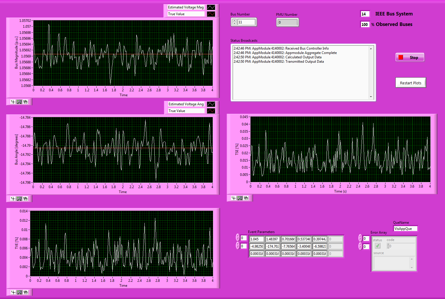
Figure B1: Front panel of the visualization VI for the LSE app. A 14 IEEE bus system is displayed.
Dynamic events
Dynamic IEEE Bus events use the Matlab Power System Toolbox installed during Quick Start.
- Run Matlab and type
s\_simu.- You will be asked to select a file, choose <your PARTF location>\Modules\Matlab\Events\CSVPlugin\cases\dtest_13_3phasefault.m to simulate a dynamic 3 phase fault in the bus number.
- The default values of 100 MVA and Base Frequency of 60Hz is suitable or can be changed.
- When s_simu completes, press enter to end the program. The fault is released after 0.1 s and after that, a ringdown event takes place. Now all the signals needed have been created in the Matlab workspace.
- Create a .csv input file for PARTF: in Matlab, type
s_simuToFile. This matlab program creates three different files in your My Documents\PARTF\Tests\LSE folder:
- The first file is a .tst file which will be opened in the PARTF framework.
- The second one .csv file in the ..\Inputdata folder containing the signals of each one of the PMUs.
- The last file is a reference signal waveform also in the ..\Inputdata folder. This file will be used during the analysis of the test results.
- Now you can browse and select the newly created DynamicSystem_case13_3pmus.tst In the PARTF
Test Filecontrol. Use theOpenbutton to create 3 buses. Note that theEvent Parameterscontrol now lists the relative path to the newly created .csv file. To run this test do the following: - Since a new test has been opened, the VisualiseAppLSE application will need to be reset by clicking on the
Restart Plotsbutton. - In the PARTF framework, click
Single Runin the bottom center of the panel. - To view any of the buses in the VisualizeAppLSE, select the bus in the
Bus Numbercontrol.
- Since a new test has been opened, the VisualiseAppLSE application will need to be reset by clicking on the
The Figure B2 below shows the results for this kind of event. With PMUs in the 10 and 11 locations only the 46% percent of the total number of buses can be estimated. The user can select which bus to visualize using the Bus Number control, in this case the number 8 is displayed.
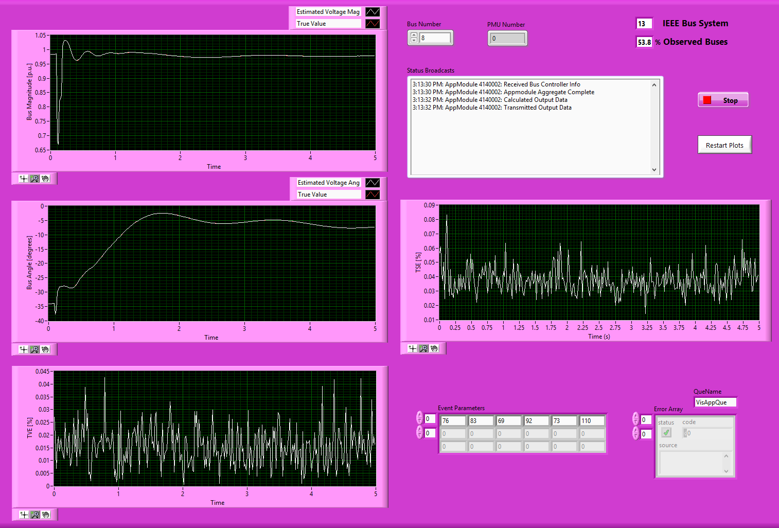
Figure B2: Front panel of the visualization VI for the LSE app. A dynamic 13 bus system is displayed.
MonteCarlo analysis
Many kinds of test can be performed using python scripts. Documentation can be found under Test Automation. Two examples of Monte Carlo Analysis are presented here:
The Effects of PMU Filtering
The first example, involves in performing a Monte Carlo simulation for a stationary IEEE bus event in order to evaluate the performance of the LSE application against the additive white Gaussian noise present in the measurements. We will use two different PMU filter types: Hamming and Blackman to see how the PMU filtering affects white Gaussian Noise rejection.
- Using the
Test Filecontrol, Browse and Select the IEEEBusSystem_case14_4pmus.tst again then clickOpen.- On the
SensorImpariment tab, change theFilterTypecontrol toHammingand click theUpdate Busbutton. Since the last bus is selected in theBus Numbercontrol each time a new test file is opened, you just changed the PMU Filter Type for the PMU on bus number 4.- Now select of each one of other 3 buses and change the
FilterTypetoHammingthen clickUpdate Busfor each. How annoying was that? (Later we will show you how to change configurations using the Monte Carlo Analysis script).
Once the bus PMUs are modified, use Monte Carlo Script control to the browse and select My Documents\PARTF\Scripts\LSE\LSEMonteCarlo.py script, then press the blue Monte Carlo button. This script will repeat the test sequence twenty times: generate the signal, generate synchrophasors and impair them as the PMU with a Hamming window would,
then run the LSE app.
The idea of this example is to run the test many times in order to gather enough data to perform a statistical analysis. This is preferable to a single test with a very long duration due to limitations in computer memory and buffer sizes. All these signals are saved in a .mat in the Output folder and again MATLAB can be used to evaluate the application performance. Please, run the \PARTF\Scripts\LSE\PlotLSENoiseTest.m. When the Select data File dialog opens, browse to ..\PARTF\Output and open the recently created data_#.mat file. As can be seen from the Figures B3 to B5 the magnitude error, the phase error and the total vector error (TVE) are plotted for each one of the voltages in the buses.
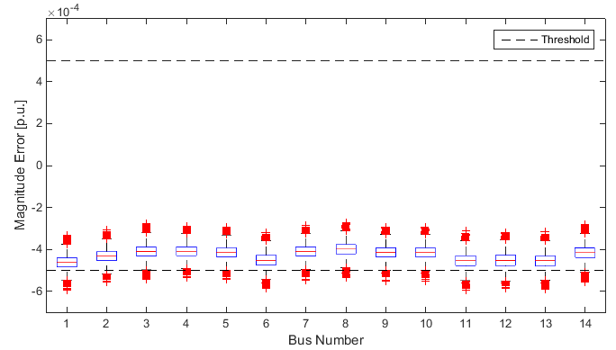
Figure B3: Boxplot [note1] of the magnitude error of all the voltages in the 14 IEEE system using a Hamming window.
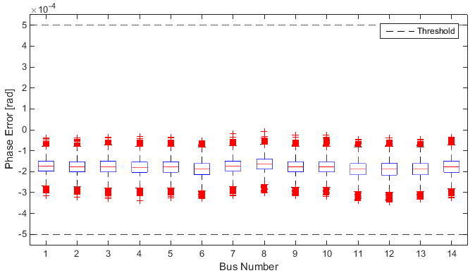
Figure B4: Boxplot of the phase error of all the voltages in the 14 IEEE system using a Hamming window.
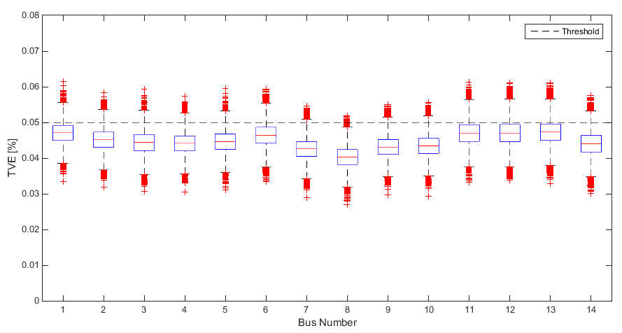
Figure B5: Boxplot of the TVE of all the voltages in the 14 IEEE system using a Hamming window.
Thresholds in each one of these magnitudes can be defined by the user to delimit the maximum error tolerated for the next step of the processing chain. As you can see the application is not complaint with expected performance.
Next we will change the PMU filter back to Blackman from Hamming. There are several ways of doing this: From the PARTF panel as we did before, from inside the matlab .tst file creation program, or using the Python Monte Carlo Script. In this example, we will use the Monte Carlo script.
In your favorite python script editing program (you can use Notepad if you do not have another) open My Documents\PARTF\Scripts\LSE\LSEMonteCarlo.py Conveniently located at line 28, you will find: PMUFilterType = ‘Hamming’ Change Hamming to Blackman. Note on lines 48 through 61 is a loop that iteratres through all the buses and loads the PMU Impairment plugin then changes the ImpairConfig.Filtertype to “PMUFilterType”. Save the file then run it again in the PARTF framework. You will notice that the FilterType on the Sensors tab changes to Blackman
Once again run the Matlab program PlotLSENoiseTest.m. You should notice a significant difference in the results:
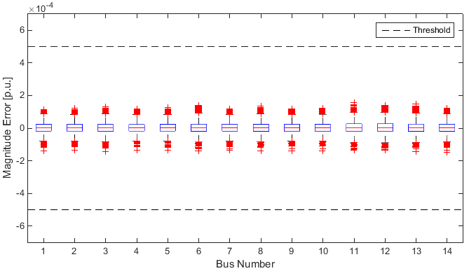
Figure B6: Boxplot of the magnitude error of all the voltages in the 14 IEEE system using a Blackman window.

Figure B7: Boxplot of the phase error of all the voltages in the 14 IEEE system using a Blackman window.
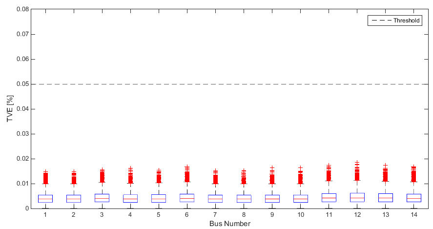
Figure B8: Boxplot of the TVE of all the voltages in the 14 IEEE system using a Blackman window.
So, as any user can expect the level of performance of the application depends on the uncertainties in the PMU measurements. The application does not include errors in the model of the system, so all the results plotted before assumes that the LSE app knows exactly the impedances between the different nodes of the network.
Observability
The second kind of test that can be performed is an observability test: How does the number of PMU in the system affect the state estimation? This next test is going to take a long time to run so you might think about starting it before lunchtime or letting it run overnight.
First we are going to edit the My Documents\PARTF\Tests\LSE\IEEEBusSystem_test_creator.m file to add a PMU for each of the 14 buses created by this program. Find line 7 and comment it out by adding a % to the front of the line. Uncomment line 8 user_pmu_list=[14 13 12 11 10 9 8 7 6 5 4 3 2 1]; by removing the %. Save and run the Matlab Program. It will create My DocumentsPARTFTestsLSEIEEEBusSystem_case14_14pmus.tst In the PARTF Framework, use the Test File control to browse and select this file. Click the Open button and 14 buses will be created. In the VisualizeAppLSE application, you can click the Restart Plots button since you just loaded a new test. Test the 14 bus system using Single Run.
In the Monte Carlo Script control, browse and select LSE\LSEPMUNumber.py. This script will repeat the same sequence of the last example 13 times with one PMU being removed with in each set of iterations. The way to reduce the PMUs is following the pmu_index variable, and as you can see the PMUs are in a descendent order. Click ‘’Monte Carlo’’ and head on home or out to lunch, this will take a while…
When the Monte Carlo simulation had finished and all the output data had been saved repeat the simulation reducing ther number of PMUs each iteration. Run the Matlab program My Documents\PARTF\Scripts\LSE\PlotLSE_PMUNumber.m. The program will as you to browse to the results file which is in My Documents\PARTF\Output\LsePmuNumber_<date_time>. This plots the results of the analysis. In this case, PMUs were removed from buses in numerical order with no consideration of the number of current channels.

Figure B9: Observability: The percentage between the estimated buses and the total number of busses in the system

Figure B10: The root average mean square error vs the number of PMUs.
If we place PMUs on buses with more current channels, we can get improved observability. Edit the LSE\LSEPMUNumber.py script to uncomment line 22 and comment out line 21. Line 22 changes the order that the PMUs that are deleted, leaving the buses with the most current channels for last. Run this revised Monte Carlo analysis to get a second set of output data. Again, take a break because this will take a while.
To compare the two sets of results, run the Matlab program My Documents\PARTF\Scripts\LSE\PlotLSE_PMUNumber_two_runs.m and select the latest set of output results first. The first value of the list corresponds to the PMU with smallest number of current channels and vice versa. We can see from the plots that using the PMUs with the most current channels improves observability.
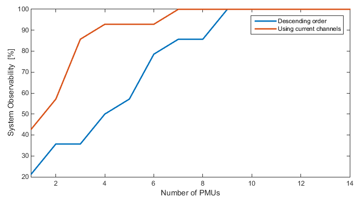
Figure B9: The percent rate between the estimated buses and the total number of buses of the system.
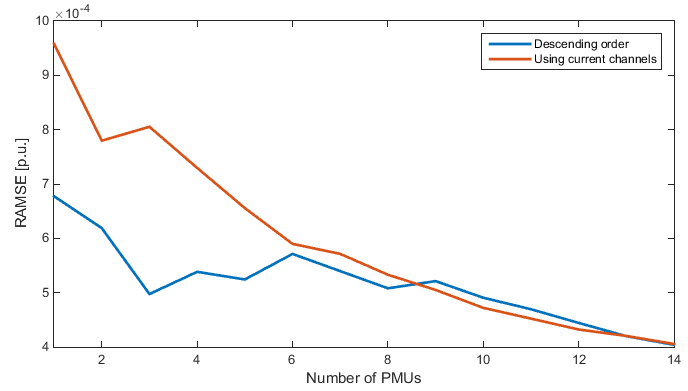
Figure B10: The root average mean square error vs the number of PMUs.
Notice that the root average mean square error, defined in , represents a metric similar to the TSE of the visualization virtual instrument, but the way that each one of them is calculated differs:
Where,
\(\varepsilon_{\text{VEi}} = \left| \left( V_{i} + \varepsilon_{\text{Vi}} \right)e^{j\left( \theta_{i} + \varepsilon_{\text{θi}} \right)} - V_{i}e^{j\theta_{i}} \right|\)
Summary of Labview Vis
EventPlugins.lvlib: IEEEBusSystemPlugin.lvclass
Parent class: EventPluginBaseClass.lvclass
Overridden Vis: GetEvtReports.vi, GetEvtSignal.vi
IEEEBusEvtPlugin.ctl: Empty, the parent class control is used.
 *GetEvtReports.vi* Icon:Inputs: IEEEBusEvtPlugin object
ClEvtConfig: T0, F0, bPosSeq
dblTimeArray
dblEvtParams
BusNumber
Outputs: IEEEBusEvtPlugin object
Timestamp
Synx
Freq
ROCOF
Description: Creates all the synchrophasors included in each one of the reports based on the eventconfiguration and the event parameters. Contains a MATLAB script block where IEEEevt.mis called. See IEEEevt.m for more details.
 *GetEvtSignal.vi* Icon:Inputs: IEEEBusEvtPlugin object
ClEvtConfig: FSamp
dblTimeArray
dblEvtParams
BusNumber
Output: IEEEBusEvtPlugin object
Signal
Description: Creates the voltage and the current waveforms. Contains a MATLAB script block wheregenIEEESignal.m is called. See genIEEESignal.m for more details.
AppPlugins.lvlib: RingdownPlugin.lvclass
 *GetAppOutput.vi* Icon:Inputs: RingdownEvtPlugin object
RingdownConfig: V index
EventConfiguration.ctl
PosSeq
Outputs: RingdownEvtPlugin object
RingdownConfig: I index
RingdownConfig: PosSeq
Description: Based on the PosSeq Boolean value, the I index is set. This index allows theGetAppOutput.vi to know where to look for the current synchrophasors values.
 *GetLSEEstimate.vi* Icon:Inputs: RingdownEvtPlugin object
RingdownConfig: V index
EventConfiguration.ctl
PosSeq
Outputs: RingdownEvtPlugin object
RingdownConfig: I index
RingdownConfig: PosSeq
Description: Based on the PosSeq Boolean value, the I index is set. This index allows theGetAppOutput.vi to know where to look for the current synchrophasors values.
 *GetPMUNumber.vi* Icon:Inputs: RingdownEvtPlugin object
RingdownConfig: V index
EventConfiguration.ctl
PosSeq
Outputs: RingdownEvtPlugin object
RingdownConfig: I index
RingdownConfig: PosSeq
Description: Based on the PosSeq Boolean value, the I index is set. This index allows theGetAppOutput.vi to know where to look for the current synchrophasors values.
 *GetMeasurementMatrix.vi* Icon:Inputs: RingdownEvtPlugin object
RingdownConfig: V index
EventConfiguration.ctl
PosSeq
Outputs: RingdownEvtPlugin object
RingdownConfig: I index
RingdownConfig: PosSeq
Description: Based on the PosSeq Boolean value, the I index is set. This index allows theGetAppOutput.vi to know where to look for the current synchrophasors values.
 *GetVoltageRef.vi* Icon:Inputs: RingdownEvtPlugin object
RingdownConfig: V index
EventConfiguration.ctl
PosSeq
Outputs: RingdownEvtPlugin object
RingdownConfig: I index
RingdownConfig: PosSeq
Description: Based on the PosSeq Boolean value, the I index is set. This index allows theGetAppOutput.vi to know where to look for the current synchrophasors values.
 *GetInterleavingSynx.vi* Icon:Inputs: RingdownEvtPlugin object
RingdownConfig: V index
EventConfiguration.ctl
PosSeq
Outputs: RingdownEvtPlugin object
RingdownConfig: I index
RingdownConfig: PosSeq
Description: Based on the PosSeq Boolean value, the I index is set. This index allows theGetAppOutput.vi to know where to look for the current synchrophasors values.
MATLAB Function descriptions
Sub-Annex– Measurement matrix calculation (H)
If we go back to the π model of a transmission line (see Fig A1) and rely on Kirchhoff’s laws, it is stated that:
Where the bar over the letter indicates that it is a phasor. If we decompose the above equation into a real and imaginary part:
Obtaining the following pair of equations:
The linear relationship that allows us to construct the matrix is observed. In the same way, the relation between the current \(I_{\text{ji}}\) can be considered, and the following scheme can be proposed:
Where \(H_{11}\) and \(H_{22}\ \)are unit matrices and \(H_{12}\) and \(H_{21}\) are null matrices. The remainder of the submatrices will contain the respective admittances according to the pair of equations described above and the equations which would correspond to the currents \(I_{\text{ji}}\).
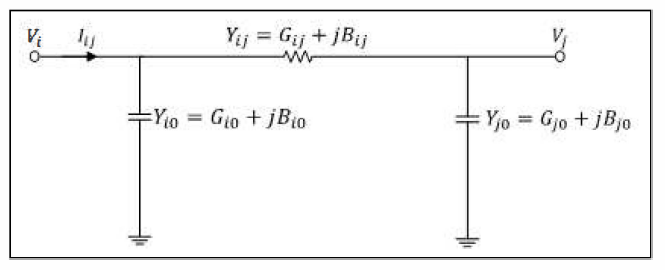
Figure B11 A11: π model of a transmission line
| [note1] | On each box, the central mark is the median, the edges of the box are the 25th and 75th percentiles, the whiskers extend to the most extreme data points the algorithm considers to be not outliers, and the outliers are plotted individually. |