Appendix C: Generator Model Validation

Introduction

Dynamic models form the basis for power system transient stability simulations. Simulation accuracy is driven, in part, by the accuracy of the individual models used to represent actual equipment installed in the field. Models are developed during the baseline testing and model creation process in close coordination between the Generator Owner and manufacturer of the components. However, model errors do exist in the dynamic cases used for planning and operating the bulk power system. These errors are introduced through component replacements, ageing, measurement error, etc., that are not captured in the updated models. Some historical disturbances can partly be attributed to model inaccuracy – post-mortem analysis using the model of expected performance has shown gross differences from actual performance. The North American Electric Reliability Corporation (NERC) Reliability Standards MOD-026-1 and MOD-027-1 seek to ensure that dynamic models are verified to ensure they accurately represent the equipment installed in the field.

Using the on-line measurement data to validate unit’s parameters has been proposed and discussed in recent years. Most of these online approaches are installing intelligent electronics devices (IEDs), such as digital fault recorders (DFRs) or phasor measurement units (PMUs), to perform the dynamic model validation test. Different techniques for using online measurement data to validate or calibrate generator model parameters were already demonstrated in the literature .

In the parameter identification step, an automatic calibration method using the extended Kalman filter (EKF) technique is used in this PMU application example. The purpose of this recursive process is to save significant effort and time from manual tuning. Publications indicate that the performance of the EKF-based method is satisfactory and is robust enough against measurement noise and parameter errors. The question which can be answered with further research using the PARTF test framework, is what is the effect of impairment of the PMU data input to the model validation?

Fundamentals of Extended Kalman Filter (EKF)

Power system dynamics can be represented generally using differential algebraic equations. From there, a state-space representation can be defined and, if we utilize the mismatch to adjust the state variables, an observer can be built. The EKF is one of the techniques for building such an observer. The discrete model formulation with a time step of $\text{Δt}$ is given by:

(1) $$\begin{split}x_{k} &= f\left( x_{k - 1},z_{k - 1},u_{k - 1}\right) \\ z_{k} &= h\left( x_{k},u_{k}\right) \\\end{split}$$

where the $x_{k}$ vector contains the state variables at k time, $\ z_{k}$ the measurements, and $u_{k}$ the input variables. Commonly $u_{k}$ is a set of measured signals used as true values for an event playback. Event playback applies measured signals to a sub-system model and simulates the model’s response for a rigorous comparison with measured response. Finally, $f$ and $h$ are nonlinear functions that define the way in which the state variables evolve and their relationship to the measurements, respectively.

The EKF is formulated as a two-step prediction-correction process. The prediction step is a time update using the difference equations represented by the $f$ function. The state variables of the next time step are estimated based on the values of the previous time step. In addition, the a-priori error covariance matrix, $P_{k|k - 1}$, is also predicted. The correction step calculates a Kalman Gain, $K_{k}$, which blends the estimated values and measured values to obtain the corrected state variables and minimize the mismatch between the estimated measurement and the actual measurement. The Kalman gain is calculated so that the a-posteriori covariance, $P_{k}$, is minimized. The equations are given below:

Prediction:

(2) $$\begin{split}x_{k|k - 1} &= f\left( x_{k - 1},z_{k - 1},u_{k - 1} \right) \\ \mathbf{P}_{k|k - 1} &= \mathbf{A}_{k}\mathbf{P}_{k - 1}{\mathbf{A}_{k}}^{T} + \mathbf{Q}_{k - 1} \\\end{split}$$

Correction:

(3) $$\begin{split}\mathbf{K}_{k} &= \mathbf{P}_{k|k - 1}{\mathbf{H}_{k}}^{T}\left( \mathbf{H}_{k}\mathbf{P}_{k|k - 1}{\mathbf{H}_{k}}^{T} + \mathbf{R}_{k} \right)^{- 1} \\ x_{k|k} &= x_{k|k - 1} + \mathbf{K}_{k}\left( z_{k} - h\left( x_{k|k - 1},u_{k} \right) \right) \\ \mathbf{P}_{k|k} &= \left( I - \mathbf{K}_{k}\mathbf{H}_{k} \right)\mathbf{P}_{k|k - 1}\end{split}$$

where $\mathbf{Q}_{k}$ is the model error covariance matrix, $\mathbf{R}_{k}$ is the measurement noise covariance matrix, and $\mathbf{A}_{k}$ and$\ \mathbf{H}_{k}$ are Jacobian matrices defined as:

(4) $$\begin{split}\mathbf{A}_{k} &= \frac{\partial f\left( x_{k - 1},z_{k - 1},u_{k - 1} \right)}{\partial x}\\ \mathbf{H}_{k} &= \frac{\partial h\left( x_{k},u_{k} \right)}{\partial x} \\\end{split}$$

Generator model

In order to model the generator unit, a classical generator model is adopted (fig.1). The discrete dynamic equations which define its behavior, and the parameters to calibrate are:

(5) $$\begin{split}\delta_{k} &= \delta_{k - 1} + bas_{\text{rad}}\ \left( \omega_{k - 1} - \omega_{0} \right)\ \text{Δt} \\ \omega_{k} &= \omega_{k - 1} + \frac{\omega_{0}\ }{2{\tilde{H}}_{k - 1}}\left( P_{m} - \frac{\text{E\ }V_{k}\sin\left( \delta_{k} - \theta_{k} \right)}{{{x^{'}}_{\text{d\ }}}_{\text{\ k} - 1}} - D\ \left( \omega_{k - 1} - \omega_{0} \right) \right)\ \text{Δt} \\ {\tilde{H}}_{k} &= {\tilde{H}}_{k - 1} \\ {{x^{'}}_{\text{d\ }}}_{k} &= {{x^{'}}_{\text{d\ }}}_{\text{\ k} - 1} \\ D_{k} &= D_{k - 1} \\\end{split}$$

Where $\delta$ represents the rotor angle, $\omega$ the angular velocity of the rotor, $\tilde{H}$ the inertia constant, $\text{ba}s_{\text{rad}}$ is a radian base normalization factor,$\ \omega_{0}$ the nominal frequency, $P_{m}$ the mechanical power, $E$ generator voltage magnitude, $V$ voltage magnitude at point of connection, $\theta$ voltage angle at point of connection, $D$ the damping coefficient and ${x^{'}}_{\text{d\ }}$ the transient reactance. Note that (5) defines the $f$ function and most of the variables are in p.u.

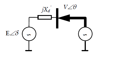
Fig. 1: Classic generator model

On the other hand, the measurements, $P/Q$ , real/reactive power at the point of connection can be calculated as:

(6) $$\begin{split}P_{k} &= \frac{\text{E\ }V_{k}\ sin(\delta_{k} - \theta_{k})}{\ {{x^{'}}_{\text{d\ }}}_{k}}\\ Q_{k} &= \frac{- V_{k}^{2} + E\ V_{k}\text{\ cos}(\delta_{k} - \theta_{k})}{\ {{x^{'}}_{\text{d\ }}}_{k}} \\\end{split}$$

Now, the $h$ function was defined by (2). Then, the state vector can be defined as $x_{k} = \left\lbrack \delta_{k}\ ,\ \omega_{k},\ H_{k},\ {{x^{'}}_{\text{d\ }}}_{k}\ ,\ D_{k} \right\rbrack^{T}\ $ , the measurement vector as $z_{k} = \left\lbrack P_{k}\ ,\ Q_{k} \right\rbrack^{T}$ and the input as $u_{k} = \left\lbrack V_{k}\ ,\ \theta_{k} \right\rbrack^{T}$.

Getting Started

Before the Generator Model Validation example can be run some first-time setup is required. This is the same setup as the Linear State Estimation example and these instructions can also be found in Quick Start

The GMV application example includes Dynamic Events. These examples require the Matlab Power System Toolbox available from The Royal Institute of Technology in Stockholm, Sweden.

• Download PSTV3, PST Data, and the Manual

• You will need to register and get a password

• As with the MatPower toolbox, unzip these into your Documents\MATLAB\Toolbox folder and set up the Matlab Path

Note that the Power System Toolbox is not open source software and cannot be redistributed.

Matlab Path

Quick Start provides instructions for setting up the matlab path to the matlab toolbox folder and all subfolders, if this was done before the PST toollbox was installed, then the path to the toolbox will also need to be added as follows:

When opening the PARTF project, a Matlab command window opens. From within this window, use the pathtool to Add with Subfolders Documents\MATLAB\ToolBox\pstv3

Example Generator Model Validation

Dynamic events

After the PST is incorporated, the user will be able to run the toolbox typing “s_simu” MATLAB function from the command window. When the user is asked to select a file, choose “<your PARTF location>\Modules\Matlab\Events\CSVPlugin\cases\d2aem.m” to simulate a dynamic 3 phase fault in the bus number 3. In this file, generation units are set as the classical generator model present in Fig. 1. The default values of 100 MVA and Base Frequency of 60Hz is suitable or can be changed. When s_simu completes, press enter to end the program. The fault is released after 0.2 s and after that, an oscillatory event takes place. Now all the signals needed have been created in the MATLAB workspace.

Create a .csv input file for PARTF: in Matlab, type s_simuToFile (Please, check in the file the values of these variables: app_sel=2; NoiseVariance=0; PMULocations=[1]). This matlab program creates three different files in your My Documents\PARTF\Tests\GMV folder:

1. The first file is a .tst file which will be opened in the PARTF

   framework.

2. The second one .csv file in the ..\Inputdata folder

   containing the signals of each one of the PMUs.

3. The last file is a reference signal waveform also in

   the ..\Inputdata folder. This file will be used during the analysis of the test results.

Now you can browse and select the newly created DynamicSystem_case13_1pmus.tst in the PARTF Test File control. Use the Open button to create the specific bus. Note that the Event Parameters control now lists the relative path to the newly created .csv file. To run this test do the following:

1. Since a new test has been opened, the VisualiseAppModelValidation

   application will need to be reset by clicking on the Restart Plots button.

2. In the PARTF framework, click Single Run in the bottom center of the

   panel.

The Figure 2 shows the results for this kind of event. Almost all the state variables are displayed. We can observe the convergence of the internal parameters of the generator model to the real values ($\tilde{H} = 6.5$, ${x^{'}}_{\text{d\ }}$=0.25, $D = 3$). The initial condition for these parameters are (${\tilde{H}}_{0} = 4.55$, ${x^{'}}_{d0\ }$=0.275, $D_{0} = 4.2$) . It is important to notice that the time zero in the visualize app corresponds to the 2s in the original reference time. The reference can be changed with the offset start time in the app configuration. The main reason of this change is to avoid the measurements values in the moment were the fault is still present in the system. The $\hat{\delta}$ is also plotted in order to check the correct operation of the method, any anomaly is easier to visualize on this variable.

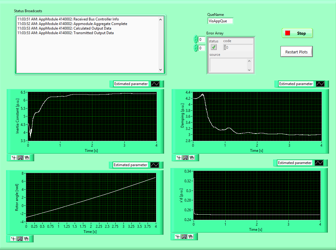
Fig. 2: Front panel of the visualization VI for the Generator Model Validation app.

It is important to mention that the results can change significantly with the interpolation factor chosen. The interpolation factor is another app config parameter. Take in account that the measurements arrive with an interarrival time defined by the reporting rate. However, the reporting time is not small enough to ensure that the linearization approach in the Kalman filter is valid. So a cubic interpolation of the phasor is used and the $\text{Δt}$ is decreased by a factor equal to $2^{\text{in}t_{\text{fac}}}\ $.

MonteCarlo analysis

Several kinds of test can be performed with the python scripts. As an example, one of them is presented in this documentation.

The initial gain matrix $\mathbf{P}_{0}$ is the co-variance matrix of the estimated state vector error. $\mathbf{P}_{k|k}$ will be updated in EKF and converge to zero if EKF works. Hence the parameters in $\mathbf{P}_{0}$ are not so much important. They only will have influence on the converge rate. Therefore, fine tuning is needed. Co-variance matrix $\mathbf{Q}_{k}$ represents the processing noise and unmolded dynamics. $\mathbf{Q}_{k}$ is less deterministic and will be considered constant at any instant of time

$\mathbf{Q}_{k} = \mathbf{Q}$. For these two matrices values similar to were used.

So the most important co-variance to define is the one which contains the covariance of the measurements $\mathbf{R}_{k}$.

Like the process covariance matrix, this matrix is ​​considered constant as a function of time $\mathbf{R}_{k} = \mathbf{R}$. So a variable called Noise Variance is defined as one of the app config parameters. With this variable the user can control the value of the diagonal elements of $\mathbf{R}$.

With the PARTF running the same .tst file of the previous example, use Monte Carlo Script control to the browse and select My Documents\PARTF\Scripts\GMV\GMVMonteCarlo.py script. Then press the blue Monte Carlo button. This script will repeat the test sequence ten times: generate the signal, generate synchrophasors and impair them as the PMU with a Blackman window would, then it runs the Model Validation app. This process is repeated for each value of the Noise Variance set. Noise Variance Set = {1e-1, 0.5e-1, 1e-2, 0.5e-2, 1e-3, 0.5e-3}

All internal signals are saved in a .mat in the DocumentsPARTFOutput folder. To evaluate the application performance, a MATLAB file has been provided in *\PARTF\Scripts\GMV\PlotGMV_MonteCarlo.m. Run this file in MATLAB and when the Select Data File dialog opens, browse to ..\PARTF\Output and open the recently created ModelGenValidation_#.mat file. As can be seen from the Figures 3 to 5 (here the sequence was repeated 1000 times), the magnitude error between the estimated parameters and the real ones are plotted for each one of the Noise Variance values.

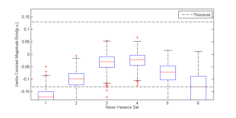
Fig. 3 Inertia constant error vs different R matrices. Threshold is equal to 2% of the reference value.

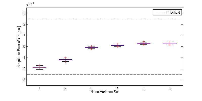
Fig. 4: Error of ${x^{'}}_{\text{d\ }}$ vs different R matrices. Threshold is equal to 1% of the reference value.

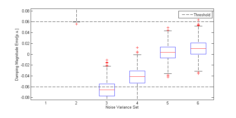
Fig. 5: Damping error vs different R matrices. Threshold is equal to 2% of the reference value.

Observing the figures, the user can conclude that a value between $0.5\ 10^{- 2}$ and $10^{- 3}$ is the optimal solution. Besides, we can assume that the error in ${x^{'}}_{\text{d }}$ is smaller than in the other cases because the initial condition is more similar to the real one.

Finally, is important to mention that the variance of the measurements is not an a-priori well known value. It is assumed that the measurements of the PMU include a specific noise distribution in the voltage magnitude and phase ($V,\theta$) and in the current magnitude and phase. For all the result display, a fixed value (almost excessive) equal to ${\sigma = 10}^{- 3}$ for the standard deviation of the AGWN of all of these values was chosen.

For further analysis of the effects of PMU filtering, as an exercize for the user, the PMU filter settings can be set by the Monte Carlo Script to simulate various PMU configurations of Class and Reporting Rate to determine effects of the noise variance on the GMV appluication.

This application example and the accompaning documentation was provided by Pablo Gabriel Marchi <pmarchi@csc.conicet.gov.ar>