Appendix A: Ringdown Example Application
Introduction
A power system is a massive system that can be perturbed by load changes, generator trips, faults or networks changes. Power system oscillations are common issues. To mitigate oscillations, oscillations should be identified and studied in a timely manner. There are two separate approaches to identify power system oscillations. The first approach is based on detailed dynamic model of the system such as eigenvalue analysis or state space modeling. The second approach is based on measurements to identify oscillation modes.
With phasor measurement unit (PMU) data collected, electromechanical oscillation modes can be identified from the synchrophasor measurements. Several measurement-based system identification methods have been proposed for PMU data-based estimation. In this documentation, we will focus on the Prony analysis. It is one of the most common measurement-based identification techniques to identify oscillatory modes, and was studied and developed by the Pacific Northwest National Laboratory (PNNL) for several years [1], [2]. The following application is based on the Dynamic System Identification (DSI) toolbox that the PNNL have implemented.
Fundamentals of Prony analysis
Consider a Linear-Time Invariant (LTI) system with the initial state of \(x(t_{0}) = x_{0}\) at the time \(t_{0}\), if the input is removed from the system, the dynamic system model can be represented as:
where \(\text{y} \in \mathbb{\text{R}}\) is defined as the output of the system, \(\text{x } \in \ \mathbb{R}^{n}\) is the state of the system, \(\text{A} \in \ \mathbb{R}^{\text{nxn}}\) and \(\text{C} \in \ \mathbb{R}^{1xn}\) are system matrices. The order of the system is defined by n. If the \(\lambda_{i}\), \(p_{i}\), and \(q_{i}\) are the i-th eigenvalues, right eigenvectors, and left eigenvectors of \(\text{n x n}\) matrix A, respectively, the system can be solved as:
Prony analysis directly estimates the parameters for the exponential terms of \(y(t)\) by defining a fitting function in a basic form of:
In other words, the output of the system is projected onto a signal consisting of a set of damped oscillations. The way in which this projection is carried out varies depending on the algorithm used. But, most of them contemplate accumulating a certain amount of samples and generating a linear prediction model, from which the roots of the characteristic polynomial of the system can be estimated.
Example ringdown application analysis
Getting started
If this is the first use of the PARTF test framework, be sure to follow the first time setup instructions in Quick Start
Open the PARTF main.vi. Select the Ringdown Event Type and the
Ringdown from Application indicators in the front panel then press the
Add Bus button. The number of buses is going to change to 1. After that
you can customize your event as you prefer. Consider the configuration
of Figure 1. An alternative method to set up the system is to press
the browse button next to the Test File control and select the
Test\Ringdown\Ringdown.tst file, then press the Open button next to
the Test File control.
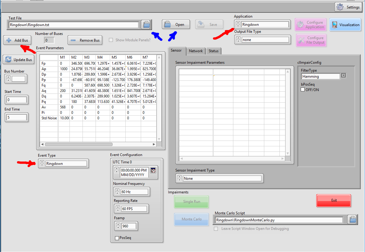
Figure 1: Front panel of the main.vi with the configuration for a simple rigndown test.
As you can observe from Figure 1 the main framework is configured to
create a ringdown event with a Start Time set to 0 seconds, End Time equal to 5 (seconds). The PMU
Reporting Rate is set to 60 frames per second with a Nominal Frequency
of 60 Hz, If a Model PMU is used for the Sensor Impairment, a sampling
frequency ( FSamp )equal to 960 Hz is used, if the impairment is not based on a
model PMU, the sampling frequency is ignored. The event default
parameters defined in the RingdownEvtPlugin.ini file are used [note1]. The
Sensor Impairment Type is changed to C37.118.1 PMU DSP Model which
basically is going to simulate the behavior of the M class PMU defined
by the IEEE 2011 standard. If changes are made to the default
configuration, the Bus must be updated with the new values: press the
Update Bus button to update the bus. If you desire to save the setup
to a test file, press the Save button and select a new test file
name or overwrite the selected one.
If a test were to be run now, all the new information would be created,
but you would not see any results. Results are viewed by using Visualization applications. One or more visualization
application can be running at the same time. To view the available
visualization applications and launch one or more of them, press the
Visualization button [note2].
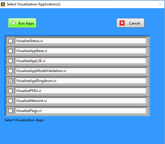
Figure 2: Visualization App selection dialog
Because the Ringdown application is active, The VisualizeAppRingdown.vi
should pre-selected. Press Run App and. a new VI emerges on the
screen. Visualization apps allow the user to observe ooperation of the PARTF while tests are running.
Without a visualization app, the tests run but there is no visual confirmation of the running tests or when they conclude.
Press the Single Run button in the PARTF frontpanel to run a single test.
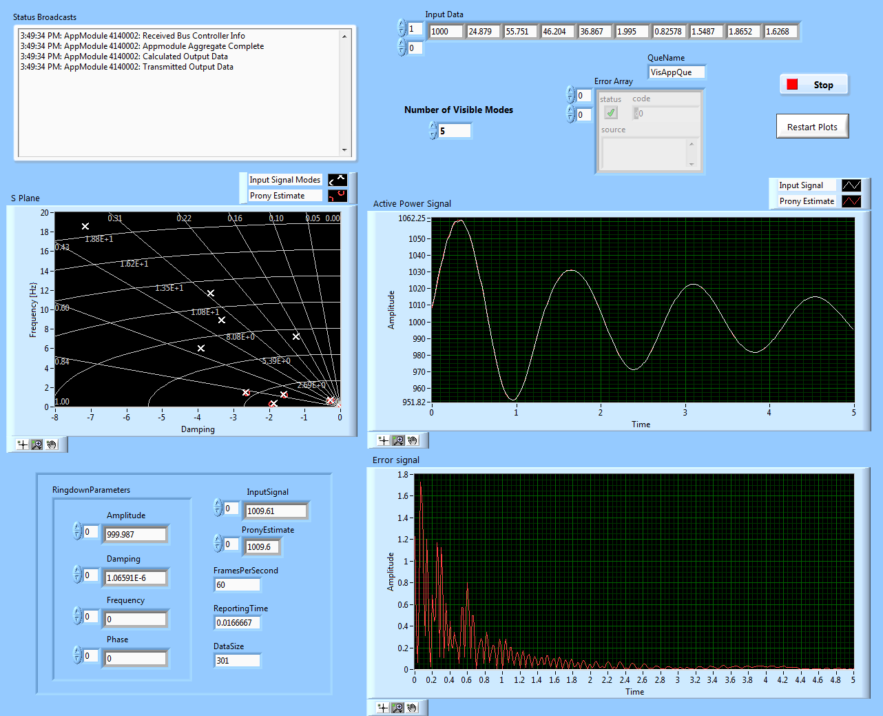
Figure 3: Front panel of the visualize.vi for a typical rigndown event .
The main features of the event are displayed on the visualization app, as you can see in figure 3. The user can observe the difference between the oscillatory modes of the input signal and the estimated ones by the Prony method in the s-plane [note3]. Furthermore, a Prony estimate signal is created form the modes and is compared with the input signal. The error signal is showing the difference between the two of them.
Simple Monte Carlo test example
The idea of this example is to understand how to use a python script to
perform Monte Carlo testing on an application and how the PMU input
signals are created. So, with the main program still running, and with
the configuration set in the example above, press the Browse button
in the Monte Carlo Script control choose the
Scripts\Ringdown\GetRingdownEvtSignal.py script then press the Monte
Carlo button. A windows command dialog will open and run the script
then close again. If you want the window to remain open after the test
(for example for debugging a script) then click the Leave Script
Window Open for Debugging checkbox. Later you can close any of these
windows left open after the test has run. Also note that closing this
command window during a test will have the effect of aborting the test.
An error message will appear in the PARTF application, but you can abort
the test without needing to close the PARTF framework.
As a result of running the GetRingdownEvtSignal.py script, a .mat and a .pkl files have been created your My Documents\PARTF\Output directory. In your My Documents\PARTF\Scripts\Ringdown\ directory, you will find a PlotRingdownSignals.m file which, when run, will create Figures 4 through 6
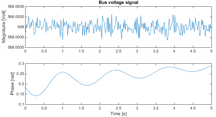
Figure 4: Matlab plot of the simulated voltage generated by the event.
If you look into the python code for GetRingdownEvtSignal.py, you can figure out that python is asking Labview for the event parameters and reports. For each one of the reports the Matlab file extracts the voltage, current, frequency and ROCOF and plots it. for details of the ringdown even, see the RngEvt.m description, the assumption that the voltage magnitude stays as a constant and that the rate of change of the current phase is defined by the Pi event parameter are corroborated. More information about PARTF test automation can be found here.
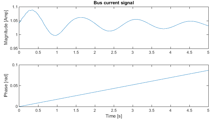
Figure 5: Matlab plot of the simulated current generated by the event.
Figure 6 shows the frequency and ROCOF signals. As you can see it contains different kinds of oscillations coming from the equation of the time derivative of the voltage phase.
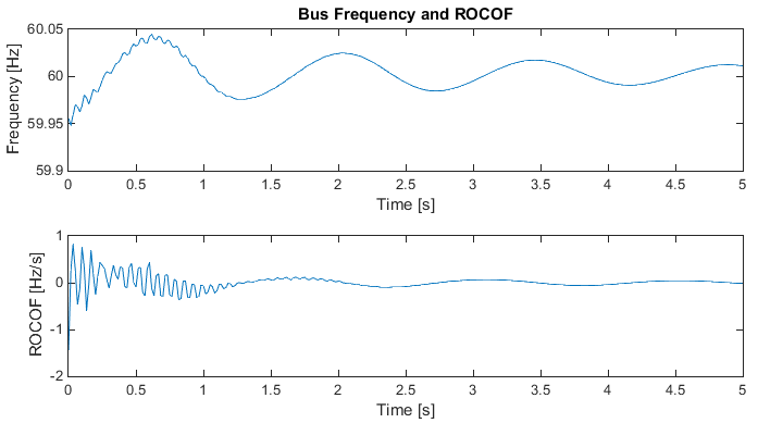
Figure 6: Matlab plot of the simulated frequency and ROCOF.
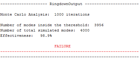
Creating a Monte Carlo analysis
Go back to the main.vi and set the End Time equal to 10. After doing
that you should remember that the Update Bus button needs to be
pressed. Then, choose the RingdownMonteCarlo.py script to start running a
sequence of events, where the only aleatory variable is the signal noise
(note that the last row of the Event Parameters has standard
deviation of noise for the M1 frequency component equal to 10e-6). At
line 12 of this script the user can select the total number of events or
iterations to be performed. After the last iteration is concluded, and
if you leave the script window open, you should see the total time that
this kind of analysis requires.
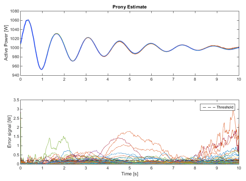
Figure 7: Set of estimated active power signals with its respective error.
The next step is to go to My Documents\PARTF\Scripts\Ringdown again
and run the PlotRingdownNoiseTest.m file in Matlab. This file is going to perform
a test to validate the application itself. Two thresholds are defined.
The first one is defined in the error signal between the active power
and the estimated one by the Prony method as you can observe from Figure
7. The error signal cannot exceed a specific value defined by the Matlab
variable error\_thres. If it does, that indicates the application is not
working as expected and we stipulate that it has a failure, as you can
see in Figure 7.
The second threshold takes place in the s plane. As you can observe from Figure 8 the first four modes with the biggest amplitudes are plotted. As you can notice the app is not working well, it looks like another mode is interfering with the result because there are a lot of points concentrated around the point {-2.5,0.3}.
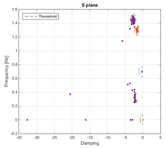
Figure 9: S plane with the oscillatory modes of the Monte Carlo analysis.
It is important to highlight that these results are different that the ones displayed by the Labview visualization tool, because in Figures 6 and 8 all the modes estimated by the Prony method are being used. In the visualizeRingdown.vi only a subgroup of visible modes is used to create the Prony estimated signal.
So, the question here is… how can we make improve the situation? Solution: Go back
to the PARTF frontpanel and click on Configure Application then change the
Linear Prediction Algorithm from total least squares via SVD to SVD with
possible rank reduction and repeat the Monte Carlo analysis. The Figures
10 through 12 show the new results. From the last figure, it is more clear that a
the thresholds in the s plane are ellipses where the radius are defined
by the Matlab freq\_std and damp\_std respectively. Although the
distribution of the output noise is unknown, the ellipses are considered
to be a good selection criterion.
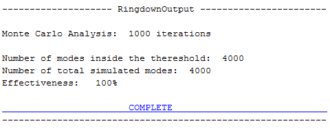
Figure 10: Command Window message, using SVD with possible rank reduction.
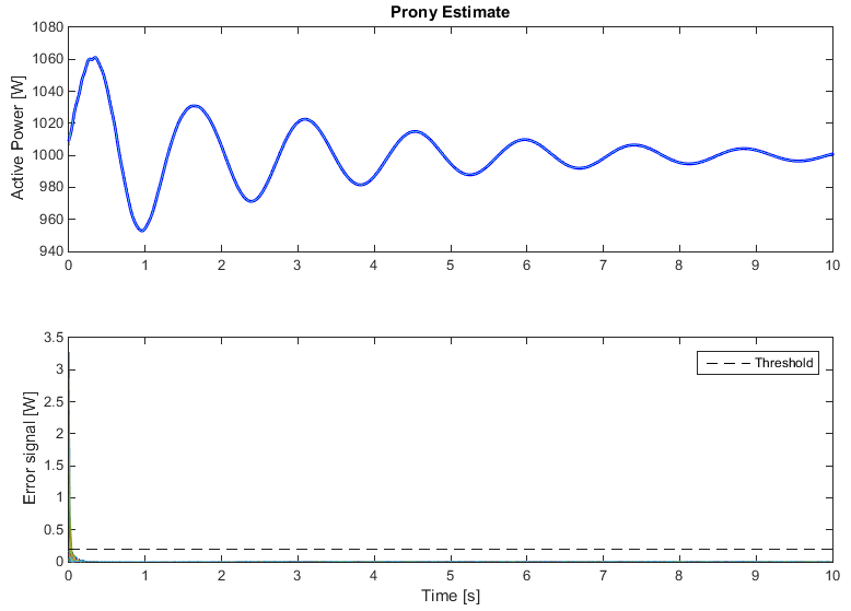
Figure 11: Set of estimated active power signals with its respective error.
The user will be able to evaluate different scenarios and corroborate that for this application the configuration of the linear predictor model is more crucial than the error coming from a PMU that is operating under the parameters of quality of the C37.118.1 IEEE standard.
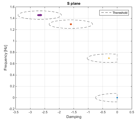
Figure 12: S plane with the oscillatory modes of the Monte Carlo analysis.
Summary of Labview Vis
EventPlugins.lvlib: RingdownEvtPlugin.lvclass
Parent class: EventPluginBaseClass.lvclass
Overridden Vis: GetEvtReports.vi, GetEvtSignal.vi
RingdownEvtPlugin.ctl: Empty, the parent class control is used.
 *GetEvtReports.vi* Icon:Inputs: RingdownEvtPlugin object
ClEvtConfig: T0, F0, bPosSeq
dblTimeArray
dblEvtParams
BusNumber
Outputs: RingdownEvtPlugin object
Timestamp
Synx
Freq
ROCOF
Description: Creates all the synchrophasors included in each one of the reports based on the eventconfiguration and the event parameters. Contains a Matlab script block where Rngevt.mis called. See Rngevt.m for more details.
 *GetEvtSignal.vi* Icon:Inputs: RingdownEvtPlugin object
ClEvtConfig: FSamp
dblTimeArray
dblEvtParams
Output: RingdownEvtPlugin object
Signal
Description: Creates the voltage and the current waveforms. Contains a Matlab script block wheregenRngSignal.m is called See genRngSignal.m for more details.
 *RgnEvtParamsErrors.vi* Icon:Empty. Reserved for future use.
AppPlugins.lvlib: RingdownPlugin.lvclass
 Parent class: AppPluginsBase.lvclass
 *AppConfig.vi* Icon:Inputs: RingdownEvtPlugin object
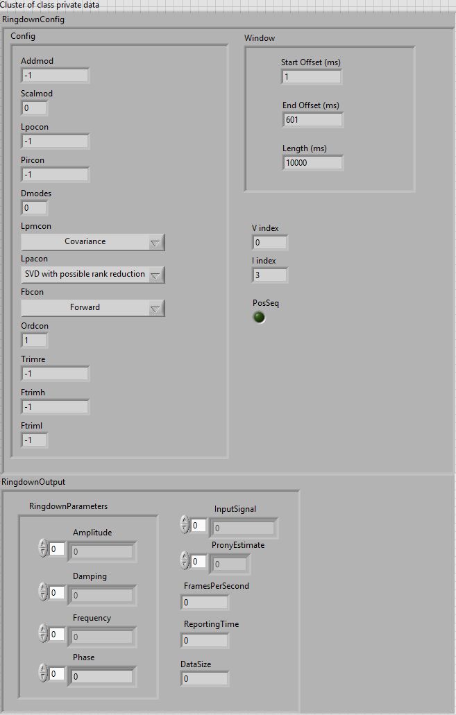
RingdownConfig: PosSeq
PronyConfiguration.ctl
Lpmcon
Lpacon
Fbcon
LPOrd
UTrimFreq
ResTrim
Outputs: RingdownEvtPlugin object
- RingdownConfig: Config.Lpmcon, Config.Lpacon, Config.Fbcon, Config.Lpocon,Config.Ftrimh, Config.Ftriml, Config.Trimre, Window.StOffset, Window.EndOffset, Window.Length, V index, I indexDescription: The Configure Application button of the front panel lunches this vi which saves all theapplication configuration that the user can modify. The significance of the variablesinvolved is described in the prgv2_6.m Matlab function.
 *WriteEvtConfig.vi* Icon:Inputs: RingdownEvtPlugin object
RingdownConfig: V index
EventConfiguration.ctl
PosSeq
Outputs: RingdownEvtPlugin object
RingdownConfig: I index
RingdownConfig: PosSeq
Description: Based on the PosSeq Boolean value, the I index is set. This index allows theGetAppOutput.vi to know where to look for the current synchrophasors values.
 *GetAppOutput.vi* Icon:Inputs: RingdownEvtPlugin object
RingdownConfig
clEvtReportArray
Outputs: RingdownEvtPlugin object
AppOutputData: ReportingTime, FramesPerSecond, InputSignal, DataSiza, PronyEstimate, RingdownParameters: Amplitude, Damping, Frequency, Phase.
Description: This vi contains a Matlab script block which calls the GetRngOutput.m file. Basically, itprocess the event report array generated by the GetEvtReports.vi or GetEvtSignal.vi, with the addition of the PMU impairs, in order to estimate all the oscillatory modes, using the configuration specified with the AppConfig.vi or the default values. From the oscillatory modes, a prony estimate signal is created also.
 *Synx2Power.vi* Icon:Inputs: RingdownEvtPlugin object
clEvtReportArray
RingdownConfig
Output: Active Power
Reactive Power
Description: From the syncrhopasors reports we select phase A to calculate the power flow throughthe branch where the PMU is connected.
 *WindowParams.vi* Icon:Inputs: RingdownEvtPlugin object
clEvtReportArray
RingdownConfig
Output: RingdownEvtPlugin object
RingdownConfig
Description: Using the difference between two consecutive timestamps, the window start offsetindex and end index are calculated form the the Window.StOffset andWindow.EndOffset time values.
 *ClusterToArray.vi* Icon:Inputs: RingdownEvtPlugin object
RingdownConfig
Output: RingdownInput
Description: The Matlab script block in the GetAppOutput.vi does not support clusters as an input, soall the rigndown configuration is converted into an array.
Matlab Function descriptions
Rngevt.m
Rngevt.m
- Purpose:To create the ringdown event reports. Each one of this reports contains a set of voltage and current synchrophasors. The time between two consecutive reports is defined by the reporting rate.
- Description/Comments:If the signal parameters define a mode above the Nyquist frequency, this mode will not keep in mind unless the internal variable nyquist_ena is settled to 0.
- Inputs:T0: Initial time (offset)F0: Nominal frequencytime: Array of times. It starts at the Start Time, and finishes at the End Time, with regularintervals defined by the reporting rate.signalparams: Matrix of doubles containing the Event Parameters specified in the front panel. The mostof them correspond to the prony_reconstruction.m input. The last three rows define themodule voltage value (V), the rate of change of the phase for the current phasor (\(\gamma_{i}\)) andthe AWG noises added in the module and the phase of the voltage and current phasors.bPosSeq: Boolean control which determines if the function adds the positive sequence to the output data.
Outputs:
timestamp: Idem time but the T0 was included.
synx: Matrix of complex containing the 3-phase voltages, the 3-phase currents and possibly the positive sequence synchrophasors.
freq: Array of doubles including the frequency of the system extracted from the voltage phase.
ROCOF: Array of doubles including the rate of change of frequency.
- AlgorithmBased on the values provided by the signalparams input, and using the prony_reconstruction.m function, the active power signal and the reactive power signal can be calculated as follows:
*V* and *I* represent the voltage and current phasors respectively. Decomposing into module and phase:
Now the voltage and the current phasors are created with the addition of the AWGN stipulated in the signalparmas matrix. At last the frequency and ROCOF are calculated as follows:
Where,
So
If the following terms are defined,
Then,
Again, for simplicity reasons the time derivatives of \(P\),\(\text{\ Q}\), \(H_{1}\) and \(H_{2}\) are not displayed.
genRngSignal.m
genRngSignal.m
Purpose: To create the ringdown event signals. These waveforms contain a set of voltage and current values at a rate equal to Fsamp (sampling frequency).
Description/Comments:
This function is very similar to the Rngevnt.m with the exception that neither the frequency nor the ROCOF and positive sequence are calculated. Finally, the output is not a phasor, it is a real waveform.
- Inputstime: Array of times. It starts at the Start Time less two times the filter order, and finishes at the End Time plus two times the filter order, with regular intervals defined by thesampling frequency.FSamp: Sampling frequencysignalparams: Matrix of doubles containing the Event Parameters specified in the front panel.
- OutputsSignal: Matrix of doubles containing the 3-phase voltages and the 3-phase currents signals.
prony_reconstruction.m
prony_reconstruction.m
Purpose: To create a time variant signal from a Prony decomposition.
- Description/Comments:It is assumed that the time goes from zero until the time defined by the total length of the signal and the time interval between samples.
Inputs
amp: Array of doubles with the amplitudes values for each one of the modes (\(A_{i}\)).phase: Array of doubles with the phases values for each one of the modes (\(\varphi_{i}\)).freq: Array of doubles with the frequencies values for each one of the modes (\(f_{i}\)).damp: Array of doubles with the dampings values for each one of the modes (\(\sigma_{i}\)).delta_t: The interval of time between samples.n_leng: Total length of the signal- Outputsprony_estimate: Vector of doubles with the real signal created from the coefficients passed as an input (\(y\)).
GetRngOutput
Purpose: To set all the variables according to the needs of the DSI toolbox and run it.
Description/Comments:
Inputs
data_in: Array of doubles with active power waveform.xcon: Array of doubles with the configuration needed for the DSI toolbox.wcon: Array of integers with the window configuration.
- Outputsdata_values: Array of doubles with the real signal created from the coefficients passed as an input (\(y\)).
data_len: Total length of the data processed
dft: Interval of time between samples
amp: Array of doubles containing the amplitudes of the oscillatory modes.
damp: Array of doubles containing the dampings of the oscillatory modes.
freq: Array of doubles containing the frequencies of the oscillatory modes.
phase: Array of doubles containing the phases of the oscillatory modes.
damp_ratio: Array of doubles with the damping ratios of each mode. The damping ration is defined as folows:
comp_time: Computing time
wrnerr: Warning flag. It indicates if the toolbox opted for aborting the prony calculation. The user will receive a null output.
prgv2_6.m
prgv2_6
Purpose: Defines the sequence of events that the toolbox needs to run the Prony method.
Description/Comments:
It is a modified version of the original one. Some object-oriented variables, which handle error messages were deleted, as well as
Inputs
sigdat: Vector of doubles with the input signal. The active power is selected.tstep: The interval of time between the PMU reports.shftnnft: A vector with two components. The first one containing a shift variable with the numberof points to skip in each column before performing the Prony analysis, and secondcontaining the data length.impulses: Input pulse matrix. First column is the delay value and the second coulmn has the amplitude value.
known_modes: Known mode matrix. First column is damping coefficients and second is mode frequencies (in rad/sec).
xcon: Control vector. This is both an input and an output.
Variable: modes, lpocon, pircon, dmodes, lpmcon, lpacon, fbcon, ordcon, trimre, ftrimh,ftrimlmodes: Number of modes in addition to those entered in knwmod to calculate.If modes == 0 just calculate residues for knwmod.If modes < 0 automatically determine number of additional modes to calculate.
scalmode: Reserved for future use.
lpocon: Order of linear prediction.
pircon: Rank of pseudo-inverse in linear prediction.
dmodes: Number of modes identified in linear prediction.
lpmcon: Linear prediction method.
lpacon: Linear prediction algorithm.
fbcon: Forward/backward linear prediction.
ordcon: Method for mode ordering.
trimre: Residue trim level.
ftrimh: Upper trim frequency.
ftriml: Lower trim frequency.
- Outputsidentmodel: Array with identified model parameters. Mode number varies along first dimension.
Parameter type varies along second dimension. (dampf, frqrps, amp, phase, resr, resi, releng, afpe). Signal number varies along third dimension, just in case of multiple inputs.
xcon: Same as input but with all the default values set.plhs_3: Variable disable. Original used for error message.plhs_4: Variable disable. Original used for error message.
prspak.m
prspak
Purpose: To estimate all the oscillatory modes of the input signal and recreate an estimative signal from these modes.
- Description/Comments:This function is the core of the toolbox because inside of this routine all the calculations to perform the Prony analysis are made. It allows to the user select a different kind of algorithms and methods to perform the linear prediction method.
Inputs
NNFIT: Number of data points for fitting. Must > 3.
KNWCON: If = 0, perform full calculation
If = 1, only calculate residues using the provided modes.
If = 2, calculate additional poles from data and calculate residues for both the known poles and the newly identified poles.
LPOCON: Order of linear prediction. If 0, auto-calculated to be 11*NNFIT/24.
LPMCON: Linear prediction method. Default is 3.
- Correlation
- Pre-windowed
- Covariance
- Post-windowed.
FBCON: Forward/Backward linear prediction. Default is 1.
- Forward
- Forward-Backward
- Backward.
LPACON: Linear prediction algorithm. Default is 1.
- SVD with possible rank reduction
- QR reduction via LAPACK
- Total least squares via SVD
PIRCON: Rank of pseudo-inverse, must be <= LPOCON. Default is LPOCON.
QCON: Number of desired modes. Default is DMODES, i.e., the maximum number possible.
In the above input variables, defaults are activated by making the variable zero.
KNWMOD: If KNWCON=1 or KNWCON=2, this is the number of known modes.
If KNWCON is any other number, this is ignored.
SIGCON: Number of signals to be analyzed
XSIG: Data sequence (0…NNFIT-1,1…SIGCON).
TSTEP: Sample period.
FTRIML: Identified modes with an imaginary part less than FTRIML are removed after identifying
residues.
DAMP: Provided only if KNWCON<>0. Vector of the real part of continuous-time poles.
FRQRPS: Provided only if KNWCON<>0. Vector of the imaginary part of continuous-time poles.
FRQRPS: Identified imaginary part of continueous-time poles.
AMPOPT: Matrix of residue amplitudes. (1…QCON) by (1…SIGCON).
PHIOPT: Matrix of residue angles in radians. (1…QCON) by (1…SIGCON).
DMODES: Total number of modes identified in the Linear Prediction.
This is also the order of the Vandermonde solution and is usually around LPOCON/2.
WRNFLG: Vector (1…NFLG) of return warning flags.
Currently, NFLG=6. If WRNFLG(I)=1, then the warning is activated.
Element 1: Numerical solution on the linear prediction SVD may be in error.
Element 2: Numerical solution on the linear prediction QR may be in error.
Element 4: Numerical solution on the root finder may be in error.
Element 6: Numerical solution on the Vandermonde problem may be in error.
MRETR: Integer flag for fatal solution. If not equal to zero, no solution is calculated.
- no flags. Solution calculated.
- 100 NNFIT < 3, i.e., too small.
- 110 XSIG is a null signal.
- 102 QCON < 1, i.e., too small.
- 103 LPOCON < 1, i.e., too small.
- 104 TSTEP too small.
- 105 QCON too small. Try increasing QCON or set QCON < KNWMOD
Notes
| [note1] | This values corresponds to the first ten estimated modes of real measurements contributed by the Bonneville Power Administration after a transmission line was switched in and out. |
| [note2] | Visualization apps should be started after at least one bus was created.
Otherwise press the app’s restart or clear button. |
| [note3] | All these plots are conditioned by the number of visibles modes set before the single run is computed. |
Citations
| [1] | Pacific Northwest National Laboratory. (2017, 07). Dynamic System Identification Toolbox. [Online]. Available: DSIToolbox. |
| [2] |
|