RK-PR

The EOS can be given as

$${\alpha }^{\mathrm{r}}={\psi }^{(-)}-{\displaystyle \frac{a_m}{RT}}{\psi }^{(+)}$$

$${\psi }^{(-)}=-\ln (1-b_m\rho )$$

$${\psi }^{(+)}={\displaystyle \frac{\ln \left({\displaystyle \frac{{\mathrm{\Delta }}_1{b}_m\rho +1}{{\mathrm{\Delta }}_2{b}_m\rho +1}}\right)}{b_m({\mathrm{\Delta }}_1-{\mathrm{\Delta }}_2)}}$$

with the EOS fixed constants of

$${\mathrm{\Delta }}_1=\sum _i{x}_i{\delta }_{1,i}$$

$${\mathrm{\Delta }}_2=\frac{1-{\mathrm{\Delta }}_1}{1+{\mathrm{\Delta }}_1}$$

The attractive term goes like

$$a_i=a_{c,i}{\left(\frac{2}{3+T/T_{c,i}}\right)}^{k_i}$$

with quadratic mixing rules

$$a_m=\sum _i\sum _j{x}_i{x}_j(1-k_{ij})\sqrt{a_i(T)a_j(T)}$$

And the covolume also gets quadratic mixing rules

$$b_m=\sum _i\sum _j{x}_i{x}_j(1-l_{ij})(b_i+b_j)/2$$

Thus, to implement the RK-PR model in predictive mode, the following steps are required:

1. Obtain the critical parameters Tc, pc

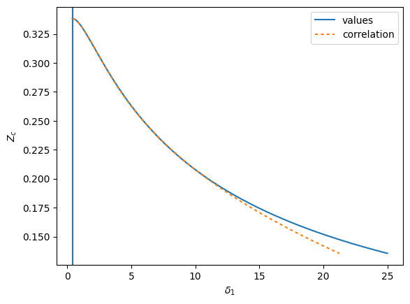
2. Solve for delta_1 from the experimental critical compressibility factor, begin with the values from the correlation

3. Solve for k by fixing the pressure at the T=0.7Tc. In the case (e.g, CO:math:`_2`) that Tt < 0.7Tc, use instead Tr=Tt/Tc

It may be necessary to adjust the values of ${\delta }_{1,i}$ and $k_i$ for an individual component to better match the behavior of more polar components.

import numpy as np
import scipy.optimize
import matplotlib.pyplot as plt
import teqp, numpy as np
import CoolProp.CoolProp as CP
import pandas

def delta1_correlation(Zc):
    # Eq. B.4 of Cismondi FPE 2005
    d1 = 0.428363
    d2 = 18.496215
    d3 = 0.338426
    d4 = 0.660000
    d5 = 789.723105
    d6 = 2.512392
    return d1 + d2*(d3-Zc)**d4 + d5*(d3-Zc)**d6

def Zc_delta1(delta1):
    # Eqs. B.1 to B.3 of Cismondi FPE 2005
    d1 = (1+delta1**2)/(1+delta1)
    y = 1 + (2*(1+delta1))**(1/3) + (4/(1+delta1))**(1/3)
    return y/(3*y + d1 - 1)

DELTA1 = np.linspace(np.sqrt(2)-1, 25, 1000)
ZZ = Zc_delta1(DELTA1)
plt.plot(DELTA1, ZZ, label='values')
DELTA1back = delta1_correlation(ZZ)
plt.axvline(np.sqrt(2)-1)
plt.plot(DELTA1back, ZZ, dashes=[2,2], label='correlation')
plt.gca().set(ylabel='$Z_c$', xlabel='$\delta_1$')
plt.legend(loc='best')
plt.show()

# for Zc in np.linspace(0.2, 0.3383, 1000):
#     resid = lambda x: Zc_delta1(x)-Zc
#     # print(resid(delta1_correlation(Zc)))
#     print(Zc, scipy.optimize.newton(resid, delta1_correlation(Zc)), delta1_correlation(Zc))

names = ['CO2', 'n-Decane']

R = 8.31446261815324
Tc  = np.array([CP.PropsSI(k,"Tcrit") for k in names])
pc  = np.array([CP.PropsSI(k,"pcrit") for k in names])
rhoc = np.array([CP.PropsSI(k,"rhomolar_critical") for k in names])
Zcexp = pc/(rhoc*R*Tc)

# Use a rescaled Zc to obtain delta_1
Zc = 1.168*Zcexp

delta_1 = [scipy.optimize.newton(lambda x: Zc_delta1(x)-Zc_, delta1_correlation(Zc_)) for Zc_ in Zc]

def solve_for_k(i, p_target, Tr):
    """
    The value of k for the i-th component is based on getting
    the right vapor pressure, so a rootfinding routing is
    used to obtain these values
    """
    def objective(k):
        j = {
            "kind": "RKPRCismondi2005",
            "model": {
                "delta_1": [delta_1[i]],
                "Tcrit / K": [Tc[i]],
                "pcrit / Pa": [pc[i]],
                "k": [k],
                "kmat": [[0.0]],
                "lmat": [[0.0]],
            }
        }
        model = teqp.make_model(j)
        T = Tr*Tc[i]
        z = np.array([1.0])
        a, b = model.get_ab(T, z)

        anc = teqp.build_ancillaries(model, Tc[i], rhoc[i], 150)
        rhoL, rhoV = model.pure_VLE_T(T, anc.rhoL(T), anc.rhoV(T), 10)
        p = T*R*rhoL*(1+model.get_Ar01(T, rhoL, z))

        return p-p_target
    return scipy.optimize.newton(objective, 2.1)

Tr = 0.7
i = 1
k_C10 = solve_for_k(i, CP.PropsSI('P','T',Tr*Tc[i],'Q',0,names[i]), Tr)

model = teqp.make_model({
    "kind": "RKPRCismondi2005",
    "model": {
        "delta_1": delta_1,
        "Tcrit / K": Tc.tolist(),
        "pcrit / Pa": pc.tolist(),
        "k": [2.23854, k_C10],
        "kmat": [[0,0],[0,0]],
        "lmat": [[0,0],[0,0]],
    }
})

# Start at both pures
for ipure in [0, 1]:
    Tc, rhoc = model.solve_pure_critical(300, 5000, {"alternative_pure_index":ipure, "alternative_length": 2})
    z = np.array([0.0, 0.0]); z[ipure] = 1.0
    pc = Tc*R*rhoc*(1+model.get_Ar01(Tc, rhoc, z))
    plt.plot(Tc, pc/1e5, 'o')

    opt = teqp.TCABOptions(); opt.polish=True; opt.verbosity=100; opt.integration_order=5; opt.rel_err=1e-10; opt.abs_err=1e-10
    trace = model.trace_critical_arclength_binary(Tc, z*rhoc, options=opt)
    df = pandas.DataFrame(trace)
    plt.plot(df['T / K'], df['p / Pa']/1e5)

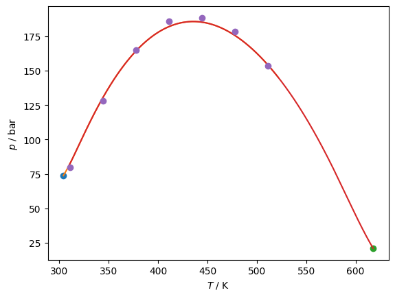
# Overlay the data from Reamer and Sage, Cismondi additional data points not present in Reamer and Sage
Tc_K = [310.928, 344.261, 377.594, 410.928, 444.261, 477.594, 510.928]
pc_kPa = np.array([7997.92, 12824.25, 16492.26, 18560.69, 18836.48, 17836.74, 15333.94])
plt.plot(Tc_K, pc_kPa/1e2, 'o')

plt.gca().set(xlabel='$T$ / K', ylabel='$p$ / bar');