Processing the 2-D NMR data

Imports

#Python modules for numerics and scientific computing
import numpy as np
import pandas as pd
import scipy as sp
import math

#scikit-learn
import sklearn.preprocessing as skpp
import sklearn.decomposition as skdecomp

#Matplotlib
%matplotlib inline
import matplotlib
import matplotlib.pyplot as plt
import matplotlib.colors as mcolors
import matplotlib.lines as mlines
import matplotlib.patches as mpatches

import mab_utils
import plot_utils as plu
#import tqdm

import interlab as inl
import pickle

Data Scaling

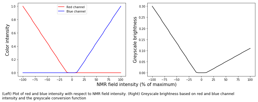
Here, we define the contour lines that are used for contour mapping, and also the scaling function that will scale the NMR intensity map into a suitable function for interlab

#Contours for contour mapping
#Contours go from 2.5 to 35 in logarithmic steps of 1.3 (i.e. 2.5, 2.5*1.3, 2.5*1.69, ...)
contoursp = 2.5*1.3**np.arange(0,11)
contoursn = -2.5*1.3**np.arange(0,11)[::-1]
ssi_contours = np.concatenate((contoursn,contoursp))

#Parameters that will be used for the piecewise linear interpolation
mid=0.5
crush_point = 0.05
crush_lo = mid-crush_point
crush_hi = mid+crush_point

#Piecewise-linear interpolation function for mapping
#Data  will be mapped FROM NMR intensity TO 0-to-1 color scale
interp_map = ([ssi_contours.min(),
               contoursn.max(),
               1e-15,
               contoursp.min(),
               ssi_contours.max()],
              [0,
               crush_lo,
               mid,
               crush_hi,
               1]
                        )

#Greyscale conversion function
greyscale_conversion = [0.3,0.59,0.11,0]

#Colormap for normalization
im=matplotlib.cm.ScalarMappable(cmap=mab_utils.RdBu_with_black.reversed(),)
#Needs to be reversed because red is positive, but we want red to be negative
cm = im.get_cmap()

#Shape of the data in release3
windowed_shape = (735,819)
nmr_window_region = [1.9,-0.9,9,30.5] #in units of ppm

plotsize = (6,4)

fig,axes=plu.make_grid_plot(1,2,plotsize=plotsize,
                            xlabel='NMR field intensity (% of maximum)')

#Create a vector of values at which to evaluate the colormap
cmap_range = np.linspace(0,1)
colormap_values = cm(cmap_range)
grey_values = np.dot(greyscale_conversion,colormap_values.T)

#Mapping from colormap space to NMR intensity space
nmr_intensity = 100*(2*cmap_range - 1)


axes.flatten()[0].plot(nmr_intensity,colormap_values[:,0],'r',label='Red channel',)
axes.flatten()[0].plot(nmr_intensity,colormap_values[:,2],'b',label='Blue channel',)

axes.flatten()[0].set_ylabel('Color intensity',size=15)
axes.flatten()[0].legend()

axes.flatten()[1].plot(nmr_intensity,grey_values,'k',)
axes.flatten()[1].set_ylabel('Greyscale brightness',size=15)

caption_text = ('(Left) Plot of red and blue intensity with respect to NMR ' +
'field intensity. (Right) Greyscale brightness based on red and blue channel\n' +
'intensity and the greyscale conversion function')

width,height = fig.get_size_inches()

t = fig.text(0,-0.25/height,caption_text,size=12,va='top')

normalization_colormap = mab_utils.RdBu_with_white.reversed()

im=matplotlib.cm.ScalarMappable(cmap=normalization_colormap,)
cma = im.get_cmap()
cm_inset = im.get_cmap()
cma = cm

plotsize = (6,4)

inset_start_x = 0.4;inset_width = -0.5
inset_start_y = 22.5;inset_height = -2.25

file = './release3/new_ext/089-D2C-S-U-600-1894-104-37C.ft2'

fig,axes=plu.make_grid_plot(1,2,plotsize=plotsize)#plt.subplots(figsize=(6,4))
mab_utils.nmr_color_scaled(file,fig,axes,cm_inset,cm,extent=nmr_window_region,
                           inset_start=(inset_start_x,inset_start_y),
                           inset_width=inset_width,inset_height=inset_height,
                           colormap_spine_color='k',
                           shape=windowed_shape,interp_map=interp_map,
                          )

# fig,axes=plu.make_grid_plot(1,2,plotsize=plotsize)#plt.subplots(figsize=(6,4))
# mab_utils.nmr_color_scaled(file,fig,axes,cm,cm,extent=[1.9,-0.9,9,30.5],
#                            inset_start=(inset_start_x,inset_start_y),
#                            inset_width=inset_width,inset_height=inset_height,
#                            colormap_spine_color='w',
#                            shape=windowed_shape,interp_map=interp_map,
#                           )

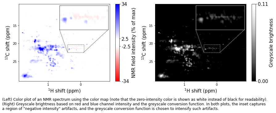
caption_text = ('(Left) Color plot of an NMR spectrum using the color map (note that ' +
                'the zero-intensity color is shown as white instead of black for ' +
                'readability). \n(Right) Greyscale brightness based on red and blue ' +
                'channel intensity and the greyscale conversion function. In both plots, ' +
                'the inset captures \na region of "negative intensity" artifacts, and ' +
                'the greyscale conversion function is chosen to intensify such artifacts.'
               )

width,height = fig.get_size_inches()

t = fig.text(0,-0.25/height,caption_text,size=12,va='top')

Reading data and metadata

Read the spectral metadata table and load it into a pandas dataframe.

metadata_table = mab_utils.read_all_metadata(metadata_file='release3/meta.tab',
                                             raw_data_path='./release3/new_ext/')

/home/local/NIST/dsheen/nistmab/mab_utils.py:118: FutureWarning: read_table is deprecated, use read_csv instead, passing sep='\t'.
  comment='#',

Read the expert scores. These scores represent the visual assessment of the spectra. 0 is a “good” spectrum, 1 is a spectrum that has noticable flaws but is still usable for scientific purposes, and 2 is a spectrum with serious flaws rendering it unusable.

expert_scores_table = pd.read_csv('release3/score.tab',
                                  skiprows=3,header=None,delim_whitespace=True)
#Extract score values from the scores table
expert_scores = expert_scores_table[0].values
#Find nonzero scores
match_expert = np.array([score>0 for score in expert_scores_table[0].values])
metadata_table['ExptScore'] = expert_scores

Display the first few entries in the metadata table so far

metadata_table.head()

	INDEX	DIR_NAME	CODE	TITLE	ExpType	ExpCode	File	ExptScore
0	1	8822	8822-010	D2C-S-U-900-8822-010-37C	800	D2C-S	./release3/new_ext/001-D2C-S-U-900-8822-010-37...	0
1	2	7425	7425-010	D2A-S-U-900-7425-010-37C	800	D2A-S	./release3/new_ext/002-D2A-S-U-900-7425-010-37...	0
2	3	7425	7425-012	D2C-S-U-900-7425-012-37C	800	D2C-S	./release3/new_ext/003-D2C-S-U-900-7425-012-37...	0
3	4	7425	7425-015	D3A-F-U-900-7425-015-37C	800	D3A-F	./release3/new_ext/004-D3A-F-U-900-7425-015-37...	0
4	5	8495	8495-010	D2A-S-U-900-8495-010-37C	800	D2A-S	./release3/new_ext/005-D2A-S-U-900-8495-010-37...	0

Read the raw spectral data into a dictionary, along with the spectral titles.

#Indices to split by
full_indices = ['ExpCode','ExpType','DIR_NAME']
split_point = 2 #This means ExpCode and ExpType will form the keys that will split the data

fulldata,full_data_dict,titles_dict = mab_utils.read_all_data(metadata_table,
                                        full_indices,
                                        split_point,
                                        shape=windowed_shape)

Processing the data

Process the raw spectral data using the color map and the greyscale conversion function.

#Empty container
data_dict = dict()
thresh = 0
#Not actually using a threshold, but keep it in the code logic in case we decide later

for description,nmrdata in full_data_dict.items():

    nmrprocessed = []
    for rawdata in nmrdata:
        #Crush values below threshold to 0
        data=np.zeros_like(rawdata)
        data[np.abs(rawdata)>thresh] = rawdata[np.abs(rawdata)>thresh]

        #Convert to colormap and greyscale-equivalent
        data,data_colors = mab_utils.colorize(data,interp_map,cm)

        #Check for zero and negative values
        data = inl.fix_spectrum(data)

        data = data/data.sum() #Sum-normalize

        #np.dot spits out a 1-D vector, need to add another axis
        nmrprocessed += [data[:,np.newaxis]]
    nmrprocessed = np.concatenate(nmrprocessed,axis=1).T
    data_dict[description] = nmrprocessed

Preparing the interlab_py analysis

Create the interlab_py project object

Create the interlab_py object, as described in Sheen, et al.

exp_keys = list(titles_dict.keys())

jeffries = r'Symmetric Kullback-Liebler'

nmr_distance_metrics = [dict(metric=r'Hellinger',function=inl.metrics.hellinger_hyp),
                        dict(metric=jeffries,function=inl.metrics.jeffries),
                       ]

mab_project = inl.Project(distance_metrics=nmr_distance_metrics,
                         Sample_names=exp_keys,Data_set_names=titles_dict,
                         data=data_dict,rawdata=full_data_dict)

Group E1-F-600 has fewer than 3 measurements, not creating
Group E1-F-800 has fewer than 3 measurements, not creating
Group E1A-F-800 has fewer than 3 measurements, not creating
Group E1C-S-800 has fewer than 3 measurements, not creating

Calculate interspectral distances

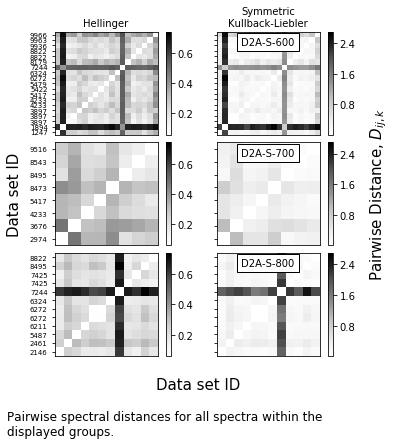
Pairwise interspectral distance is calculated using the symmetric Kullback-Liebler divergence,

\[d_{SKL}(x,y) = \frac{1}{2} \left( \sum_{i} \left( x_i - y_i \right) \log \frac{x_i}{y_i} \right)\]

where \(x\) and \(y\) are any two spectra and \(x_i\) and \(y_i\) are the elements of those spectra.

mab_project.set_distances()

plot_range = ['D2A-S-600',
              'D2A-S-700',
              'D2A-S-800',
             ]

f = mab_project.plot_distance_fig(plot_range=plot_range,
                                  plot_data=False,
                                  ylabel_buffer=0.4,rightlabel_buffer=0.4)

for ax,label in zip(f.axes[1::2],plot_range):
    ax.text(0.5,0.95,label,ha='center',va='top',transform=ax.transAxes,bbox=dict(facecolor='w'),)

caption_text = ('Pairwise spectral distances for all spectra within the \ndisplayed groups.')

width,height = f.get_size_inches()

t = f.text(0,-0.25/height,caption_text,size=12,va='top',)

Save data tables and Interlab project

metadata_table.to_hdf('metadata_table_raw.h5',key='NMR_2D_raw',mode='w')

with open('mAb_interlab_project.sav','wb') as f:
    pickle.dump(mab_project,f)

with open('mab_analysis_accessories.sav','wb') as f:
    pickle.dump((windowed_shape,jeffries,full_indices,split_point,ssi_contours,interp_map),f)