examples.diffusion.newtonCoupled

Perform Newton iterations to solve non-linear equations.

>>> import fipy as fp
>>> from matplotlib import pyplot as plt

We wish to solve a single diffusion equation in 1D, where the diffusion coefficient is a nonlinear function of the solution variable.

(1)\[\begin{split}\begin{aligned} \frac{\partial A}{\partial t} &= \nabla\cdot\left[ \left(3 + A^3\right)\left(2 + B^2\right)\nabla A \right] \\ \frac{\partial B}{\partial t} &= \nabla\cdot\left[A^5\nabla B\right] \end{aligned}\end{split}\]

>>> mesh = fp.Grid1D(nx=100, dx=1.)
>>> A = fp.CellVariable(mesh=mesh, name="A", value=0., hasOld=True)
>>> B = fp.CellVariable(mesh=mesh, name="B", value=0., hasOld=True)

>>> Aface = A.faceValue
>>> Bface = B.faceValue
>>> Aeq = (fp.TransientTerm(var=A)
...        == fp.DiffusionTerm(coeff=(3 + Aface**3)*(2 + Bface**2), var=A))
>>> Beq = (fp.TransientTerm(var=B) == fp.DiffusionTerm(coeff=A**5, var=B))
>>> eq = Aeq & Beq

subject to the boundary conditions

\[\begin{split}\begin{aligned} A &= 1\qquad\text{at \(x = 0\)} \\ B &= 2\qquad\text{at \(x = 100\)} \end{aligned}\end{split}\]

>>> A.constrain(1., where=mesh.facesLeft)
>>> B.constrain(2., where=mesh.facesRight)

We start by solving with fixed-point iterations. We’ll collect residuals for comparison later. We’ll take multiple sweeps of this non-linear equation for a single, large time step.

>>> fixedPoint = []
>>> A.updateOld()
>>> B.updateOld()
>>> for sweep in range(20):
...     res = eq.sweep(dt=1000.)
...     fixedPoint.append([sweep, res])

Store the result for comparison later:

>>> Afixed = A.copy()
>>> Afixed.name = "A fixed point"
>>> Bfixed = B.copy()
>>> Bfixed.name = "B fixed point"

As in examples.diffusion.newton, given an approximate set of solutions \(\mathbf{x}\) to the equations \(\mathbf{F}(\mathbf{x})\), we apply Newton’s method to seek an improved set of solutions \(\mathbf{x} + \delta\mathbf{x}\) by applying a first order Taylor expansion

(2)\[\mathbf{F}(\mathbf{x} + \delta \mathbf{x}) \approx \mathbf{F}(\mathbf{x}) + \left.\delta \mathbf{F}\right\rvert_\mathbf{x} \approx 0\]

where \(\delta\) is a variation operator, such that for

(3)\[\begin{split}\mathbf{F}(\mathbf{x}) \equiv \left\{ \begin{aligned} \frac{\partial A}{\partial t} &= \nabla\cdot\left[ \left(3 + A^3\right)\left(2 + B^2\right)\nabla A \right] \\ \frac{\partial B}{\partial t} &= \nabla\cdot\left[A^5\nabla B\right] \end{aligned} \right.\end{split}\]

then

(4)\[\begin{split} \delta \mathbf{F} \equiv \left\{ \begin{aligned} \frac{\partial\, \delta A}{\partial t} &= \nabla\cdot\left[ \delta A \, 3 A^2\left(2 + B^2\right)\nabla A \right] \\ &\qquad {} + \nabla\cdot\left[ \left(3 + A^3\right)\left(2 + B^2\right)\nabla \delta A \right] \\ &\qquad {} + \nabla\cdot\left[ \delta B\, 2 B \left(3 + A^3\right)\nabla A \right] \\ \frac{\partial \, \delta B}{\partial t} &= \nabla\cdot\left[\delta A\,5 A^4\nabla B\right] + \nabla\cdot\left[A^5\nabla \delta B\right] \end{aligned} \right.\end{split}\]

We can now use Eqs. (3) and (4) to solve Eq. (2) for \(\delta A\) and \(\delta B\).

>>> dA = fp.CellVariable(mesh=mesh, name=r"$\delta A$", hasOld=True)
>>> dB = fp.CellVariable(mesh=mesh, name=r"$\delta B$", hasOld=True)
>>> dAeq = ((fp.TransientTerm(var=dA)
...          == fp.ConvectionTerm(coeff=3*Aface**2*(2+Bface**2)*A.faceGrad, var=dA)
...          + fp.DiffusionTerm(coeff=(3 + Aface**3)*(2 + Bface**2), var=dA)
...          + fp.ConvectionTerm(coeff=2*Bface*(3 + Aface**3)*A.faceGrad, var=dB))
...         + fp.ResidualTerm(equation=Aeq))
>>> dBeq = ((fp.TransientTerm(var=dB)
...          == fp.ConvectionTerm(coeff=5*Aface**4*B.faceGrad, var=dA)
...          + fp.DiffusionTerm(coeff=Aface**5, var=dB))
...         + fp.ResidualTerm(equation=Beq))
>>> deq = dAeq & dBeq

Note

Because Aeq and Beq were used in coupled form for the fixed-point solution, and are now used in decoupled form for their residuals, we must clear out their cached matrices. This was not necessary in examples.diffusion.newton because the matrix did not change shape between calculating the uncoupled fixed point solution and the uncoupled Newton residual.

>>> eq.reset()

At Dirichlet boundaries, the value of \(A\) or \(B\) is determined by the boundary condition and their variations are zero:

>>> dA.constrain(0., where=mesh.facesLeft)
>>> dB.constrain(0., where=mesh.facesRight)

We reset the solutions and their variations and, again, collect residuals for later comparison.

>>> A.value = 0.
>>> B.value = 0.
>>> dA.value = 0.
>>> dB.value = 0.

Note

It’s necessary to reset the variation in the solution at every sweep, to prevent Newton increments from the previous linearization from entering the new off-diagonal Jacobian terms as explicit source values (thanks to @sbtristan98!).

>>> newton = []
>>> A.updateOld()
>>> B.updateOld()
>>> dA.updateOld()
>>> dB.updateOld()
>>> for sweep in range(20):
...     dA.value = 0.
...     dB.value = 0.
...     res = deq.sweep(dt=1000.)
...     A.value = A.value + dA.value
...     B.value = B.value + dB.value
...     newton.append([sweep, res, max(abs(dA)), max(abs(dB))])

and examine the result:

>>> Anewton = A.copy()
>>> Anewton.name = "A Newton"
>>> Bnewton = B.copy()
>>> Bnewton.name = "B Newton"

The solutions agree, although not terribly well.

>>> print(Anewton.allclose(Afixed, rtol=2e-4))
True
>>> print(Bnewton.allclose(Bfixed, rtol=1e-2))
True

>>> if __name__ == '__main__':
...     viewer = fp.Viewer(vars=(Afixed, Anewton, Bfixed, Bnewton))
...     viewer.plot()

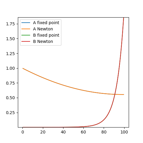
Solutions vs position for a coupled non-linear diffusion problem evolved by fixed point and Newton iteration. Fixed point and Newton solutions overlie each other.

Convert residual lists into arrays

>>> fixedPoint = fp.numerix.array(fixedPoint)
>>> newton = fp.numerix.array(newton)

and compare convergence, observing that the Newton iterations converge to a much smaller residual than the fixed point iterations:

>>> print(fixedPoint[10, 1] > 1e-5)
True

>>> print(newton[10, 1] < 1e-13)
True

>>> if __name__ == '__main__':
...     plt.figure()
...     plt.semilogy(fixedPoint[...,0], fixedPoint[..., 1], label="fixed point")
...     plt.semilogy(newton[...,0], newton[..., 1], label="Newton")
...     plt.ylabel("residual")
...     plt.xlabel("sweep")
...     plt.legend()
...     plt.show()

>>> if __name__ == '__main__':
...     input("Coupled equation fixed-point vs Newton iteration. Press <return> to proceed...")

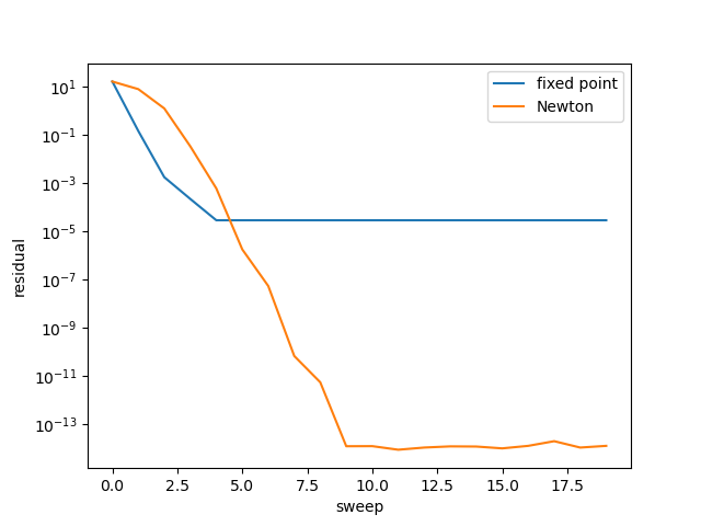
Convergence of coupled non-linear diffusion problem evolved by fixed point and Newton iterations.

Last updated on Oct 01, 2026. Created using Sphinx 9.1.0.