examples.diffusion.newton

Perform Newton iterations to solve non-linear equations.

>>> import fipy as fp
>>> from matplotlib import pyplot as plt

We wish to solve a single diffusion equation in 1D, where the diffusion coefficient is a nonlinear function of the solution variable.

(1)\[\frac{\partial C}{\partial t} = \nabla\cdot\left[ \left(3 + C^3\right)\left(2 + C^2\right)\nabla C \right]\]

>>> mesh = fp.Grid1D(nx=100, dx=1.)
>>> C = fp.CellVariable(name="C", mesh=mesh, value=0., hasOld=True)

>>> Cface = C.faceValue
>>> eq = (fp.TransientTerm(var=C)
...       == fp.DiffusionTerm(coeff=(3 + Cface**3) * (2 + Cface**2), var=C))

subject to the boundary condition

\[C = 1\qquad\text{at \(x = 0\)}\]

>>> C.constrain(1., where=mesh.facesLeft)

We start by solving with fixed-point iterations. We’ll collect residuals for comparison later. We’ll take multiple sweeps of this non-linear equation for a single, large time step.

>>> fixedPoint = []
>>> C.updateOld()
>>> for sweep in range(20):
...     res = eq.sweep(dt=1000.)
...     fixedPoint.append([sweep, res])

Store the result for comparison later:

>>> Cfixed = C.copy()
>>> Cfixed.name = "C fixed point"

If \(\mathbf{x}\) is an approximate solution to a set of equations \(\mathbf{F}(\mathbf{x})\), such that

\[\mathbf{F}(\mathbf{x}) \approx 0\]

Newton’s method is a technique where we seek a new solution \(\mathbf{x} + \delta \mathbf{x}\) that hopefully has a smaller residual for

\[\mathbf{F}(\mathbf{x} + \delta \mathbf{x}) \approx 0.\]

We apply a first order Taylor expansion

(2)\[\mathbf{F}(\mathbf{x} + \delta \mathbf{x}) \approx \mathbf{F}(\mathbf{x}) + \left.\delta \mathbf{F}\right\rvert_\mathbf{x} \approx 0\]

where \(\delta\) is a variation operator, such that for

(3)\[\mathbf{F}(\mathbf{x}) = \mathbf{F}(C) \equiv \left\{ \frac{\partial C}{\partial t} = \nabla\cdot\left[\left(3 + C^3\right)\left(2 + C^2\right)\nabla C\right] \right\}\]

then, by the chain rule,

(4)\[\begin{split}\begin{aligned} \delta \mathbf{F}(C) &\equiv \delta\left\{ \frac{\partial C}{\partial t} = \nabla\cdot\left[ \left(3 + C^3\right)\left(2 + C^2\right)\nabla C \right] \right\} \\ &\equiv \frac{\partial\, \delta C}{\partial t} = \nabla\cdot\left\{ \delta C\left[ 3 C^2 \left(2 + C^2\right) + \left(3 + C^3\right) 2 C \right] \nabla C \right\} \\ &\qquad\qquad {} + \nabla\cdot\left[ \left(3 + C^3\right)\left(2 + C^2\right)\nabla \delta C \right] \end{aligned}\end{split}\]

Note

There’s probably a more proper way to get here via variational derivatives and the Euler-Lagrange equation, but it’s leaving me with a couple of extra terms that blow up the solution. More rigorous derivations are welcome.

We can now use Eqs. (3) and (4) to solve Eq. (2) for \(\delta C\).

>>> deltaC = fp.CellVariable(mesh=mesh, name=r"$\delta C$", hasOld=True)
>>> newtonEq = ((fp.TransientTerm(var=deltaC)
...              == fp.ConvectionTerm(coeff=(3*Cface**2*(2 + Cface**2)
...                                          + (3 + Cface**3)*2*Cface) * C.faceGrad,
...                                   var=deltaC)
...              + fp.DiffusionTerm(coeff=(3 + Cface**3) * (2 + Cface**2), var=deltaC))
...             + fp.ResidualTerm(equation=eq, underRelaxation=1.))

At a Dirichlet boundary, the value of \(C\) is determined by the boundary condition and its variation is zero:

>>> deltaC.constrain(0., where=mesh.facesLeft)

We reset the solution and its variation and, again, collect residuals for later comparison.

>>> C.value = 0
>>> deltaC.value = 0

Note

It’s necessary to reset the variation in the solution at every sweep, to prevent Newton increments from the previous linearization from entering the new off-diagonal Jacobian terms as explicit source values (thanks to @sbtristan98!).

>>> newton = []
>>> C.updateOld()
>>> deltaC.updateOld()
>>> for sweep in range(20):
...     deltaC.value = 0.
...     res = newtonEq.sweep(dt=1000.)
...     C.value = C.value + deltaC.value
...     newton.append([sweep, res, max(abs(deltaC))])

and examine the result:

>>> Cnewton = C.copy()
>>> Cnewton.name = "C Newton"

The solutions agree, although not terribly well.

>>> print(Cnewton.allclose(Cfixed, rtol=4e-3))
True

>>> if __name__ == '__main__':
...     viewer = fp.Viewer(vars=(Cfixed, Cnewton),
...                        datamin=0.,
...                        datamax=1.)
...     viewer.plot()

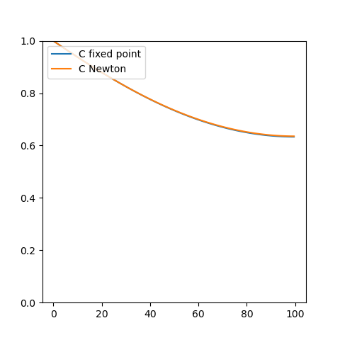
Solution vs position for a coupled non-linear diffusion problem evolved by fixed point and Newton iteration. Fixed point and Newton solutions overlie each other.

Convert residual lists into arrays

>>> fixedPoint = fp.numerix.array(fixedPoint)
>>> newton = fp.numerix.array(newton)

and compare convergence, observing that the Newton iterations converge to a much smaller residual than the fixed point iterations:

>>> print(fixedPoint[10, 1] > 1e-4)
True

>>> print(newton[10, 1] < 1e-13)
True

>>> if __name__ == '__main__':
...     plt.figure()
...     plt.semilogy(fixedPoint[...,0], fixedPoint[..., 1], label="fixed point")
...     plt.semilogy(newton[...,0], newton[..., 1], label="Newton")
...     plt.ylabel("residual")
...     plt.xlabel("sweep")
...     plt.legend()
...     plt.show()

>>> if __name__ == '__main__':
...     input("Single equation fixed-point vs Newton iteration. Press <return> to proceed...")

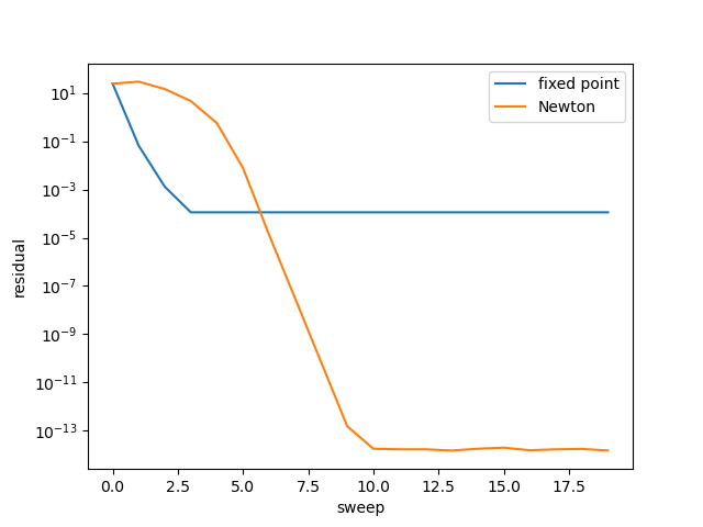
Convergence of non-linear diffusion problem evolved by fixed point and Newton iterations.

Last updated on Oct 01, 2026. Created using Sphinx 9.1.0.