examples.elphf.phase

A simple 1D example to test the setup of the phase field equation.

We rearrange Eq. (1) to

\[\begin{split}\frac{1}{M_\xi}\frac{\partial \xi}{\partial t} &= \kappa_{\xi}\nabla^2 \xi + \frac{\epsilon'(\xi)}{2}\left(\nabla\phi\right)^2 \\ &\qquad - \left[ p'(\xi) \Delta\mu_n^\circ + g'(\xi) W_n \right] - \sum_{j=2}^{n-1} C_j \left[ p'(\xi) \Delta\mu_{jn}^\circ + g'(\xi) W_{jn} \right] - C_{\text{e}^{-}} \left[ p'(\xi) \Delta\mu_{\text{e}^{-}}^\circ + g'(\xi) W_{\text{e}^{-}} \right]\end{split}\]

The single-component phase field governing equation can be represented as

\[\frac{1}{M_\xi} \frac{\partial \xi}{\partial t} = \kappa_\xi \nabla^2 \xi - 2\xi(1-\xi)(1-2\xi) W\]

where \(\xi\) is the phase field, \(t\) is time, \(M_\xi\) is the phase field mobility, \(\kappa_\xi\) is the phase field gradient energy coefficient, and \(W\) is the phase field barrier energy.

We solve the problem on a 1D mesh

>>> from fipy import CellVariable, Grid1D, TransientTerm, DiffusionTerm, ImplicitSourceTerm, Viewer
>>> from fipy.tools import numerix

>>> nx = 400
>>> dx = 0.01
>>> L = nx * dx
>>> mesh = Grid1D(dx = dx, nx = nx)

We create the phase field

>>> phase = CellVariable(mesh = mesh, name = 'xi')
>>> phase.mobility = numerix.inf
>>> phase.gradientEnergy = 0.025

Although we are not interested in them for this problem, we create one field to represent the “solvent” component (1 everywhere)

>>> class ComponentVariable(CellVariable):
...     def copy(self):
...         new = self.__class__(mesh = self.mesh,
...                              name = self.name,
...                              value = self.value)
...         new.standardPotential = self.standardPotential
...         new.barrier = self.barrier
...         return new

>>> solvent = ComponentVariable(mesh = mesh, name = 'Cn', value = 1.)
>>> solvent.standardPotential = 0.
>>> solvent.barrier = 1.

and one field to represent the electrostatic potential (0 everywhere)

>>> potential = CellVariable(mesh = mesh, name = 'phi', value = 0.)
>>> permittivityPrime = 0.

We’ll have no substitutional species and no interstitial species in this first example

>>> substitutionals = []
>>> interstitials = []

>>> for component in substitutionals:
...     solvent -= component

>>> phase.equation = TransientTerm(coeff = 1/phase.mobility) \
...     == DiffusionTerm(coeff = phase.gradientEnergy) \
...     - (permittivityPrime / 2.) \
...        * potential.grad.dot(potential.grad)

>>> enthalpy = solvent.standardPotential
>>> barrier = solvent.barrier
>>> for component in substitutionals + interstitials:
...     enthalpy += component * component.standardPotential
...     barrier += component * component.barrier

We linearize the source term in the same way as in examples.phase.simple.

>>> mXi = -(30 * phase * (1. - phase) * enthalpy \
...         +  4 * (0.5 - phase) * barrier)
>>> dmXidXi = (-60 * (0.5 - phase) * enthalpy + 4 * barrier)
>>> S1 = dmXidXi * phase * (1 - phase) + mXi * (1 - 2 * phase)
>>> S0 = mXi * phase * (1 - phase) - phase * S1

>>> phase.equation -= S0 + ImplicitSourceTerm(coeff = S1)

Note

Adding a Term to an equation formed with == will add to the left-hand side of the equation and subtracting a Term will add to the right-hand side of the equation

We separate the phase field into electrode and electrolyte regimes

>>> phase.setValue(1.)
>>> phase.setValue(0., where=mesh.cellCenters[0] > L / 2)

Even though we are solving the steady-state problem (\(M_\phi = \infty\)) we still must sweep the solution several times to equilibrate

>>> from builtins import range
>>> for step in range(10):
...     phase.equation.solve(var = phase, dt=1.)

Since we have only a single component \(n\), with \(\Delta\mu_n^\circ = 0\), and the electrostatic potential is uniform, Eq. (1) reduces to

\[\frac{1}{M_\xi}\frac{\partial \xi}{\partial t} = \kappa_{\xi}\nabla^2 \xi - g'(\xi) W_n\]

which we know from examples.phase.simple has the analytical solution

\[\xi(x) = \frac{1}{2}(1 - \tanh\frac{x - L/2}{2d})\]

with an interfacial thickness \(d = \sqrt{\kappa_{\xi}/2W_n}\).

We verify that the correct equilibrium solution is attained

>>> x = mesh.cellCenters[0]

>>> d = numerix.sqrt(phase.gradientEnergy / (2 * solvent.barrier))
>>> analyticalArray = (1. - numerix.tanh((x - L/2.)/(2 * d))) / 2.

>>> phase.allclose(analyticalArray, rtol = 1e-4, atol = 1e-4).value
1

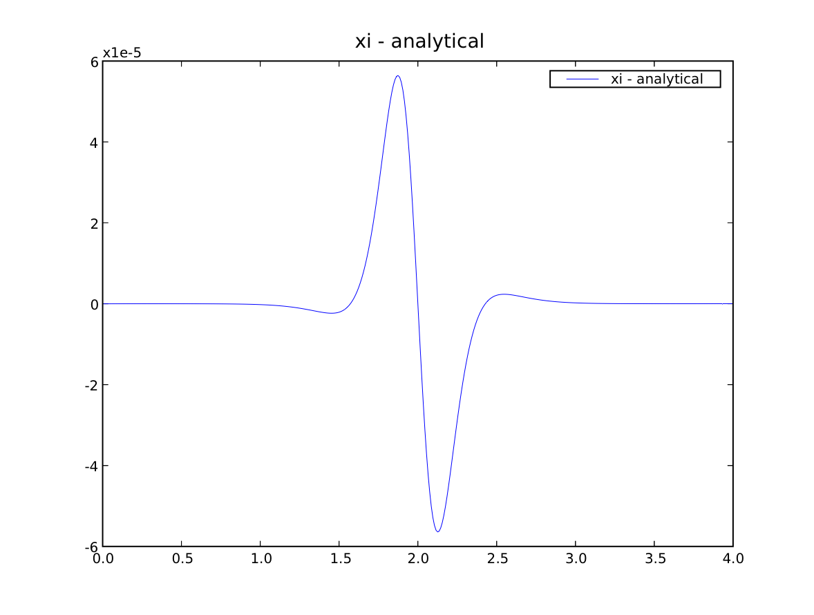
If we are running interactively, we plot the error

>>> if __name__ == '__main__':
...     viewer = Viewer(vars = (phase - \
...         CellVariable(name = "analytical", mesh = mesh,
...                      value = analyticalArray),))
...     viewer.plot()

Last updated on Jun 26, 2024. Created using Sphinx 7.1.2.