 FiPy
FiPyexamples.cahnHilliard.mesh2DCoupled
Solve the Cahn-Hilliard problem in two dimensions.
Warning
This formulation has serious performance problems and is not automatically tested. Specifically, for non-trivial mesh sizes, (obsolete) Pysparse required enormous amounts of memory, Trilinos cannot solve the coupled form, and PETSc cannot solve the vector form.
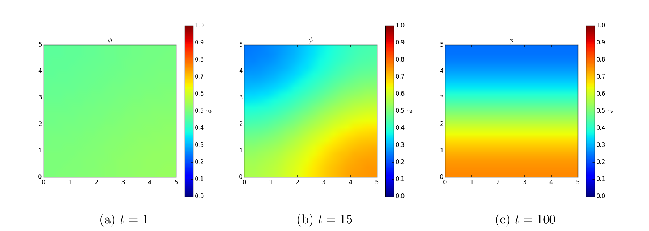
The spinodal decomposition phenomenon is a spontaneous separation of an initially homogeneous mixture into two distinct regions of different properties (spin-up/spin-down, component A/component B). It is a “barrierless” phase separation process, such that under the right thermodynamic conditions, any fluctuation, no matter how small, will tend to grow. This is in contrast to nucleation, where a fluctuation must exceed some critical magnitude before it will survive and grow. Spinodal decomposition can be described by the “Cahn-Hilliard” equation (also known as “conserved Ginsberg-Landau” or “model B” of Hohenberg & Halperin)
where \(\phi\) is a conserved order parameter, possibly representing alloy composition or spin. The double-well free energy function \(f = (a^2/2) \phi^2 (1 - \phi)^2\) penalizes states with intermediate values of \(\phi\) between 0 and 1. The gradient energy term \(\epsilon^2 \nabla^2\phi\), on the other hand, penalizes sharp changes of \(\phi\). These two competing effects result in the segregation of \(\phi\) into domains of 0 and 1, separated by abrupt, but smooth, transitions. The parameters \(a\) and \(\epsilon\) determine the relative weighting of the two effects and \(D\) is a rate constant.
We can simulate this process in FiPy with a simple script:
>>> from fipy import CellVariable, Grid2D, GaussianNoiseVariable, DiffusionTerm, TransientTerm, ImplicitSourceTerm, Viewer
>>> from fipy.tools import numerix
(Note that all of the functionality of NumPy is imported along with FiPy, although much is augmented for FiPy's needs.)
>>> if __name__ == "__main__":
...     nx = ny = 20
... else:
...     nx = ny = 10
>>> mesh = Grid2D(nx=nx, ny=ny, dx=0.25, dy=0.25)
>>> phi = CellVariable(name=r"$\phi$", mesh=mesh)
>>> psi = CellVariable(name=r"$\psi$", mesh=mesh)
We start the problem with random fluctuations about \(\phi = 1/2\)
>>> noise = GaussianNoiseVariable(mesh=mesh,
...                               mean=0.5,
...                               variance=0.01).value
>>> phi[:] = noise
FiPy doesn’t plot or output anything unless you tell it to:
>>> if __name__ == "__main__":
...     viewer = Viewer(vars=(phi,), datamin=0., datamax=1.)
We factor the Cahn-Hilliard equation into two 2nd-order PDEs and place them in canonical form for FiPy to solve them as a coupled set of equations.
The source term in \(\psi\), \(\frac{\partial f}{\partial \phi}\), is
expressed in linearized form after Taylor expansion at \(\phi=\phi_{\text{old}}\),
for the same reasons discussed in examples.phase.simple.
We need to perform the partial derivatives
manually.
>>> D = a = epsilon = 1.
>>> dfdphi = a**2 * phi * (1 - phi) * (1 - 2 * phi)
>>> dfdphi_ = a**2 * (1 - phi) * (1 - 2 * phi)
>>> d2fdphi2 = a**2 * (1 - 6 * phi * (1 - phi))
>>> eq1 = (TransientTerm(var=phi) == DiffusionTerm(coeff=D, var=psi))
>>> eq2 = (ImplicitSourceTerm(coeff=1., var=psi)
...        == ImplicitSourceTerm(coeff=d2fdphi2, var=phi) - d2fdphi2 * phi + dfdphi
...        - DiffusionTerm(coeff=epsilon**2, var=phi))
>>> eq3 = (ImplicitSourceTerm(coeff=1., var=psi)
...        == ImplicitSourceTerm(coeff=dfdphi_, var=phi)
...        - DiffusionTerm(coeff=epsilon**2, var=phi))
>>> eq = eq1 & eq2
Because the evolution of a spinodal microstructure slows with time, we use exponentially increasing time steps to keep the simulation “interesting”. The FiPy user always has direct control over the evolution of their problem.
>>> dexp = -5
>>> elapsed = 0.
>>> if __name__ == "__main__":
...     duration = 100.
... else:
...     duration = .5e-1
>>> while elapsed < duration:
...     dt = min(100, numerix.exp(dexp))
...     elapsed += dt
...     dexp += 0.01
...     eq.solve(dt=dt)
...     if __name__ == "__main__":
...         viewer.plot()
>>> from fipy import input
>>> if __name__ == '__main__':
...     input("Coupled equations. Press <return> to proceed...")
These equations can also be solved in FiPy using a vector equation. The variables \(\phi\) and \(\psi\) are now stored in a single variable
>>> var = CellVariable(mesh=mesh, elementshape=(2,))
>>> var[0] = noise
>>> if __name__ == "__main__":
...     viewer = Viewer(name=r"$\phi$", vars=var[0,], datamin=0., datamax=1.)
>>> D = a = epsilon = 1.
>>> v0 = var[0]
>>> dfdphi = a**2 * v0 * (1 - v0) * (1 - 2 * v0)
>>> dfdphi_ = a**2 * (1 - v0) * (1 - 2 * v0)
>>> d2fdphi2 = a**2 * (1 - 6 * v0 * (1 - v0))
The source terms have to be shaped correctly for a vector. The implicit source coefficient has to have a shape of (2, 2) while the explicit source has a shape (2,)
>>> source = (- d2fdphi2 * v0 + dfdphi) * (0, 1)
>>> impCoeff = d2fdphi2 * ((0, 0),
...                        (1., 0)) + ((0, 0),
...                                    (0, -1.))
This is the same equation as the previous definition of eq, but now in a vector format.
>>> eq = (TransientTerm(((1., 0.),
...                     (0., 0.))) == DiffusionTerm([((0.,          D),
...                                                   (-epsilon**2, 0.))])
...                                   + ImplicitSourceTerm(impCoeff) + source)
>>> dexp = -5
>>> elapsed = 0.
>>> while elapsed < duration:
...     dt = min(100, numerix.exp(dexp))
...     elapsed += dt
...     dexp += 0.01
...     eq.solve(var=var, dt=dt)
...     if __name__ == "__main__":
...         viewer.plot()
>>> print(numerix.allclose(var, (phi, psi)))
True