examples.cahnHilliard.mesh2D

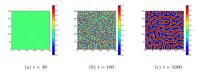
The spinodal decomposition phenomenon is a spontaneous separation of an initially homogeneous mixture into two distinct regions of different properties (spin-up/spin-down, component A/component B). It is a “barrierless” phase separation process, such that under the right thermodynamic conditions, any fluctuation, no matter how small, will tend to grow. This is in contrast to nucleation, where a fluctuation must exceed some critical magnitude before it will survive and grow. Spinodal decomposition can be described by the “Cahn-Hilliard” equation (also known as “conserved Ginsberg-Landau” or “model B” of Hohenberg & Halperin)

\[\frac{\partial \phi}{\partial t} = \nabla\cdot D \nabla\left( \frac{\partial f}{\partial \phi} - \epsilon^2 \nabla^2 \phi\right).\]

where \(\phi\) is a conserved order parameter, possibly representing alloy composition or spin. The double-well free energy function \(f = (a^2/2) \phi^2 (1 - \phi)^2\) penalizes states with intermediate values of \(\phi\) between 0 and 1. The gradient energy term \(\epsilon^2 \nabla^2\phi\), on the other hand, penalizes sharp changes of \(\phi\). These two competing effects result in the segregation of \(\phi\) into domains of 0 and 1, separated by abrupt, but smooth, transitions. The parameters \(a\) and \(\epsilon\) determine the relative weighting of the two effects and \(D\) is a rate constant.

We can simulate this process in FiPy with a simple script:

>>> from fipy import CellVariable, Grid2D, GaussianNoiseVariable, TransientTerm, DiffusionTerm, ImplicitSourceTerm, LinearLUSolver, Viewer
>>> from fipy.tools import numerix

(Note that all of the functionality of NumPy is imported along with FiPy, although much is augmented for FiPy's needs.)

>>> if __name__ == "__main__":
...     nx = ny = 1000
... else:
...     nx = ny = 20
>>> mesh = Grid2D(nx=nx, ny=ny, dx=0.25, dy=0.25)
>>> phi = CellVariable(name=r"$\phi$", mesh=mesh)

We start the problem with random fluctuations about \(\phi = 1/2\)

>>> phi.setValue(GaussianNoiseVariable(mesh=mesh,
...                                    mean=0.5,
...                                    variance=0.01))

FiPy doesn’t plot or output anything unless you tell it to:

>>> if __name__ == "__main__":
...     viewer = Viewer(vars=(phi,), datamin=0., datamax=1.)

For FiPy, we need to perform the partial derivative \(\partial f/\partial \phi\) manually and then put the equation in the canonical form by decomposing the spatial derivatives so that each Term is of a single, even order:

\[\frac{\partial \phi}{\partial t} = \nabla\cdot D a^2 \left[ 1 - 6 \phi \left(1 - \phi\right)\right] \nabla \phi- \nabla\cdot D \nabla \epsilon^2 \nabla^2 \phi.\]

FiPy would automatically interpolate D * a**2 * (1 - 6 * phi * (1 - phi)) onto the faces, where the diffusive flux is calculated, but we obtain somewhat more accurate results by performing a linear interpolation from phi at cell centers to PHI at face centers. Some problems benefit from non-linear interpolations, such as harmonic or geometric means, and FiPy makes it easy to obtain these, too.

>>> PHI = phi.arithmeticFaceValue
>>> D = a = epsilon = 1.
>>> eq = (TransientTerm()
...       == DiffusionTerm(coeff=D * a**2 * (1 - 6 * PHI * (1 - PHI)))
...       - DiffusionTerm(coeff=(D, epsilon**2)))

Because the evolution of a spinodal microstructure slows with time, we use exponentially increasing time steps to keep the simulation “interesting”. The FiPy user always has direct control over the evolution of their problem.

>>> dexp = -5
>>> elapsed = 0.
>>> if __name__ == "__main__":
...     duration = 1000.
... else:
...     duration = 1000.

>>> while elapsed < duration:
...     dt = min(100, numerix.exp(dexp))
...     elapsed += dt
...     dexp += 0.01
...     eq.solve(phi, dt=dt, solver=LinearLUSolver())
...     if __name__ == "__main__":
...         viewer.plot()
...     elif (max(phi.globalValue) > 0.7) and (min(phi.globalValue) < 0.3) and elapsed > 10.:
...         break

>>> print((max(phi.globalValue) > 0.7) and (min(phi.globalValue) < 0.3))
True

Last updated on Jun 26, 2024. Created using Sphinx 7.1.2.