Including instrument line shapes in simulation and fits

Provided in the MATS v2 release are several examples highlighting MATS capabilities, which can be found in the MATS examples folder.

MATS has added the capability to simulate and fit spectra using an instrument lineshape. MATS automatically loads the slit functions defined in HAPI, but could use any slit function with the form slit_function(x, resolution) or slit_function(x, [resolutions]). MATS uses a slight variation of the HAPI convolveSpectrumSame, where the arange_ function was redefined to address an integer/float bug in the underlying np.linspace call. This implementation currently assumes an equal wavenumber spacing based on the application of the slit function calculation.

The example below simulates the same spectrum and applies the different HAPI instrument line shapes. The simulated molefraction is perturbted and then floated during a fit.

Simulate Spectra with ILS

Module import follows from the Fitting Experimental Spectra and Fitting Synthetic Spectra examples with additional details on how to simulate spectra found in Fitting Synthetic Spectra and the source documentation.

from MATS.linelistdata import linelistdata
import MATS.hapi as hapi

# Shared Simulation and Fit Parameters
IntensityThreshold = 1e-30 #intensities must be above this value to be simulated
Fit_Intensity = 1e-24#intensities must be above this value for the line to be fit
wave_range = 1.5 #range outside of experimental x-range to simulate
IntensityThreshold = 1e-30 #intensities must be above this value to be simulated
segment_column = None
order_baseline_fit = 1
etalon = {}
SNR = 5000
resolution = 0.25
molefraction = {2:0.01}
wave_min = 6320
wave_max = 6340
wave_step = 0.01

When fitting spectra, the simulated spectral range is the minimum and maximum wavenumbers in your dataset +/- an extra spectral window defined in this example by the wave_range parameter. This is used to truncate the input line list when generating the Parameter linelist used in fitting to increase the fit speed. However, this trunctation doesn’t occur when simulating spectra, which can lead to far-wing effects as the default is to calculate each transition to +/- 25 half-widths from the line center. For this example, we are truncating input line list used for the simulation to match the fit simulation window. Alternatively, the wave_range parameter could be increased substantially to include these far-wing impacts.

PARAM_LINELIST = linelistdata['CO2_30012']
PARAM_LINELIST = PARAM_LINELIST[(PARAM_LINELIST['nu'] <= wave_max + wave_range) & (PARAM_LINELIST['nu']>= wave_min - wave_step)]

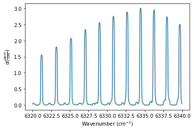
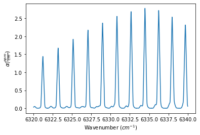
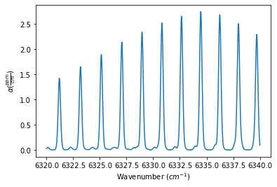
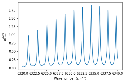
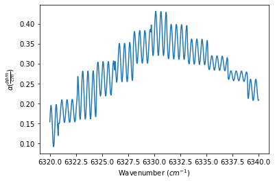
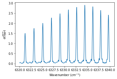
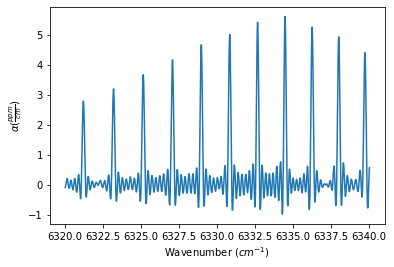
The Spectrum object definitions below show how to use the ILS_function, ILS_resolution, and ILS_wing (defines the length of the ILS slit function to use in the convolution, such that the length is +/- ILS_wing / spectrum stepsize) to define the ILS function. The outputs below show the generated spectrum for each ILS_function

spec_rectangular =  MATS.simulate_spectrum(PARAM_LINELIST, wave_min, wave_max, wave_step,
                             SNR = SNR, baseline_terms = [0], temperature = 22.85,
                             pressure = 150,
                              filename = 'Rectangular',
                            molefraction =  {2:0.01} , ILS_function = SLIT_RECTANGULAR, ILS_resolution = resolution, ILS_wing = 10)

spec_triangular=  MATS.simulate_spectrum(PARAM_LINELIST, wave_min, wave_max, wave_step,
                             SNR = SNR, baseline_terms = [0], temperature = 22.85,
                             pressure = 150,
                              filename = 'Triangular',
                            molefraction =  {2:0.01}, ILS_function = SLIT_TRIANGULAR, ILS_resolution = resolution, ILS_wing = 10)

spec_gaussian =  MATS.simulate_spectrum(PARAM_LINELIST, wave_min, wave_max, wave_step,
                             SNR = SNR, baseline_terms = [0], temperature = 22.85,
                             pressure = 150,
                              filename = 'Gaussian',
                            molefraction =  {2:0.01}, ILS_function = SLIT_GAUSSIAN, ILS_resolution = resolution, ILS_wing = 10)

spec_dispersion =  MATS.simulate_spectrum(PARAM_LINELIST, wave_min, wave_max, wave_step,
                             SNR = SNR, baseline_terms = [0], temperature = 22.85,
                             pressure = 150,
                              filename = 'Dispersion',
                            molefraction =  {2:0.01}, ILS_function = SLIT_DISPERSION, ILS_resolution = resolution, ILS_wing = 10)

spec_cosinus =  MATS.simulate_spectrum(PARAM_LINELIST, wave_min, wave_max, wave_step,
                             SNR = SNR, baseline_terms = [0], temperature = 22.85,
                             pressure = 150,
                              filename = 'Cosinus',
                            molefraction =  {2:0.01}, ILS_function = SLIT_COSINUS, ILS_resolution = resolution, ILS_wing = 10)

spec_diffraction =  MATS.simulate_spectrum(PARAM_LINELIST, wave_min, wave_max, wave_step,
                             SNR = SNR, baseline_terms = [0], temperature = 22.85,
                             pressure = 150,
                              filename = 'Diffraction',
                            molefraction =  {2:0.01}, ILS_function = SLIT_DIFFRACTION, ILS_resolution = resolution, ILS_wing = 10)

spec_michelson =  MATS.simulate_spectrum(PARAM_LINELIST, wave_min, wave_max, wave_step,
                             SNR = SNR, baseline_terms = [0], temperature = 22.85,
                             pressure = 150,
                              filename = 'Michelson',
                            molefraction =  {2:0.01}, ILS_function = SLIT_MICHELSON, ILS_resolution = resolution, ILS_wing = 10)

Generate Dataset and Fit Parameters

The dataset and fit parameters are generated with instances of the Dataset and

Generate_FitParam_File classes. Additionally, the initial CO2 molefraction is perturbed within 2% of the simulated mole fraction.

SPECTRA = MATS.Dataset([ spec_rectangular, spec_triangular, spec_gaussian, spec_dispersion, spec_cosinus,
                            spec_diffraction, spec_michelson],  'ILS Study', PARAM_LINELIST)
BASE_LINELIST = SPECTRA.generate_baseline_paramlist()

BASE_LINELIST['molefraction_CO2'] = BASE_LINELIST['molefraction_CO2'].values*(1 + np.random.normal(loc = 0, scale =1, size = len(BASE_LINELIST['molefraction_CO2']))*(2/100)) #Adjust the mole fraction of each sample by a mole fraction of random value normally distributed 2%




FITPARAMS = MATS.Generate_FitParam_File(SPECTRA, PARAM_LINELIST, BASE_LINELIST,
                                        lineprofile = 'SDNGP', linemixing = True,
                                           fit_intensity = Fit_Intensity, threshold_intensity = IntensityThreshold,
                                           nu_constrain = True, sw_constrain = True, gamma0_constrain = True, delta0_constrain = True,
                                            aw_constrain = True, as_constrain = True,
                                            nuVC_constrain = True, eta_constrain =True, linemixing_constrain = True)


FITPARAMS.generate_fit_param_linelist_from_linelist(vary_nu = {2:{1:False, 2:False, 3:False}}, vary_sw = {2:{1:False, 2:False, 3:False}},
                                                 vary_gamma0 = {2:{1: False, 2:False, 3: False}}, vary_n_gamma0 = {2:{1:False}},
                                                 vary_delta0 = {2:{1:False, 2:False, 3: False}}, vary_n_delta0 = {2:{1:False}},
                                                 vary_aw = {2:{1: False, 2:False, 3: False}}, vary_n_gamma2 = {2:{1:False}},
                                                 vary_as = {2:{1:False}}, vary_n_delta2 = {2:{1:False}},
                                                 vary_nuVC = {2:{1:False}}, vary_n_nuVC = {2:{1:False}},
                                                 vary_eta = {}, vary_linemixing = {2:{1:False}})

FITPARAMS.generate_fit_baseline_linelist(vary_baseline = False, vary_molefraction = {2:True}, vary_ILS_res = False)

In the Generate_FitParam_File.generate_fit_baseline_linelist() function, in addition to the normal baseline parameters the ILS resolution parameters are also fittable parameters. Additionally, this is coded in such a way that each ILS_function has a unique resolution parameter. This allows for different spectra to have different ILS functions and the baseline linelist table adequately accounts for this. Subset of a Generate_FitParam_File.generate_fit_baseline_linelist() output highlights this. While floating the resolution parameters is possible, it should be done with caution as all other parameters are dependent on this value, so correlation and poor fits are likely.

Spectrum Number    SLIT_RECTANGULAR_res_0    SLIT_RECTANGULAR_res_0_err    SLIT_RECTANGULAR_res_0_vary    SLIT_MICHELSON_res_0
1                      0.25                                          0                                                         False                                                  0
. . .
7                      0                                             0                                                         False                                                  0.25

Fit Data

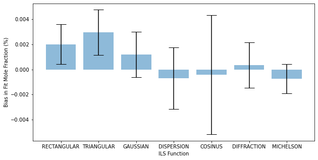
In this example only the sample concentration is allowed to float, which is a spectrum dependent parameter. At this SNR all of the results yield fit mole fractions very similar to the simulated value. The plot below shows the relative Bias in the fit mole fraction with error bars equal to the relative fit uncertainty for each ILS. Note that this is only one iteration and not generalizable.

fit_data = MATS.Fit_DataSet(SPECTRA,'Baseline_LineList', 'Parameter_LineList', minimum_parameter_fit_intensity = Fit_Intensity)
params = fit_data.generate_params()
for param in params:
 if ('_res_' in param) and (params[param].vary == True):
     params[param].set(min = 0.01)

result = fit_data.fit_data(params)
print (result.params.pretty_print())
fit_data.residual_analysis(result, indv_resid_plot=True)
fit_data.update_params(result)
SPECTRA.generate_summary_file(save_file = True)