Fitting and Simulating isotopes and molecules not in HITRAN
Provided in the MATS v2 release are several examples highlighting MATS capabilities, which can be found in the MATS examples folder.
HITRAN’s focus is on atmospherically relevent molecules. This was the original focus of MATS, however recent feature development has allowed for adaption of to include non-HITRAN molecules.
The example shows how to supplement the HITRAN isotope list and then use that in simulations and fits. This example uses Mercury as an examaple case This example uses Mercury as an example case.
Append to the HITRAN isotope list to include desired isotopes
Module import follows from the Fitting Experimental Spectra and Fitting Synthetic Spectra examples.
The add_to_HITRANstyle_isotope_list() function allows you to ammend a given isotope list to include additional molecules and/or isotopes using the HITRAN-style molcule_id, local_isotope id, and global isotope id parameterization. This function has some checks to verify expected behavior
- if the molecule id and isotope id are in the initial isotope line list, it will return ‘Already entry with that molec_id and local_iso_id. This result will write over that entry.
- if the molecule id is in the initial isotope list it will return ‘This is being added as a new isotope of molecule name. Proceed if that was the intention.
- if the global isotope id is already in the isotope list it will return, ‘There is another entry with this global isotope id. Consider changing the value for consistency’
Mercury line shape parameters are not included in the HITRAN database. The code below uses add_to_HITRANstyle_isotope_list() function to add 10 Mercury isotopes to the HITRAN isotope list. This is saved in a new isotope list called HITRAN_Hg_isolist that can be used in simulating and fitting spectra. The HITRAN isotope list provides the HITRAN molecule and global ids that are already in use.
from MATS.hapi import ISO
from MATS import add_to_HITRANstyle_isotope_list

HITRAN_Hg_isolist = add_to_HITRANstyle_isotope_list(input_isotope_list = ISO, molec_id = 100, local_iso_id = 1,
                                                 global_isotope_id = 200, iso_name = '196',
                                                 abundance = 0.0015, mass = 195.96581, mol_name = 'Hg')
HITRAN_Hg_isolist = add_to_HITRANstyle_isotope_list(input_isotope_list = HITRAN_Hg_isolist, molec_id = 100, local_iso_id = 2,
                                                 global_isotope_id = 201, iso_name = '198',
                                                 abundance = 0.1004, mass =197.96674, mol_name = 'Hg')
HITRAN_Hg_isolist = add_to_HITRANstyle_isotope_list(input_isotope_list = HITRAN_Hg_isolist, molec_id = 100, local_iso_id = 3,
                                                 global_isotope_id = 202, iso_name = '199A',
                                                 abundance = 0.1694, mass =198.96825, mol_name = 'Hg')
HITRAN_Hg_isolist = add_to_HITRANstyle_isotope_list(input_isotope_list = HITRAN_Hg_isolist, molec_id = 100, local_iso_id = 4,
                                                 global_isotope_id = 203, iso_name = '199B',
                                                 abundance = 0.1694, mass =198.96825, mol_name = 'Hg')
HITRAN_Hg_isolist = add_to_HITRANstyle_isotope_list(input_isotope_list = HITRAN_Hg_isolist, molec_id = 100, local_iso_id = 5,
                                                 global_isotope_id = 204, iso_name = '200',
                                                 abundance = 0.2314, mass =199.96825, mol_name = 'Hg')
HITRAN_Hg_isolist = add_to_HITRANstyle_isotope_list(input_isotope_list = HITRAN_Hg_isolist, molec_id = 100, local_iso_id = 6,
                                                 global_isotope_id = 205, iso_name = '201a',
                                                 abundance = 0.1317, mass =200.97028, mol_name = 'Hg')
HITRAN_Hg_isolist = add_to_HITRANstyle_isotope_list(input_isotope_list = HITRAN_Hg_isolist, molec_id = 100, local_iso_id = 7,
                                                 global_isotope_id = 206, iso_name = '201b',
                                                 abundance = 0.1317, mass =200.97028, mol_name = 'Hg')
HITRAN_Hg_isolist = add_to_HITRANstyle_isotope_list(input_isotope_list = HITRAN_Hg_isolist, molec_id = 100, local_iso_id = 8,
                                                 global_isotope_id = 207, iso_name = '201c',
                                                 abundance = 0.1317, mass =200.97028, mol_name = 'Hg')
HITRAN_Hg_isolist = add_to_HITRANstyle_isotope_list(input_isotope_list = HITRAN_Hg_isolist, molec_id = 100, local_iso_id = 9,
                                                 global_isotope_id = 208, iso_name = '202',
                                                 abundance = 0.2974, mass =201.97062, mol_name = 'Hg')
HITRAN_Hg_isolist = add_to_HITRANstyle_isotope_list(input_isotope_list = HITRAN_Hg_isolist, molec_id = 100, local_iso_id = 10,
                                                 global_isotope_id = 209, iso_name = '204',
                                                 abundance = 0.0682, mass =203.97347, mol_name = 'Hg')
Generate Spectra
The simulate spectrum function is used to generate spectra (similar to in the Fitting Synthetic Spectra example), but the isotope_list variable is set to use the isotope list that was just generated opposed to using the default HITRAN isotope list defined in HAPI.
The initial parameter line list should have molecule and local isotope ids that correspond to the new isotope list. The mole fraction definition should also use the appropriate mole fraction id. The same would be true for the abundance_ratio_MI term if the sample was not at natural abundance.
PARAM_LINELIST = pd.read_csv('Hg_Linelist.csv')
#Generic Fit Parameters
wave_range = 1.5 #range outside of experimental x-range to simulate
IntensityThreshold = 1e-30 #intensities must be above this value to be simulated
Fit_Intensity = 1e-17 #intensities must be above this value for the line to be fit
order_baseline_fit = 0
tau_column = 'Absoprtion Coefficient (ppm/cm)' # Mean tau/us
freq_column = 'Frequency (cm-1)' # Total Frequency /MHz
pressure_column = 'Pressure (Torr)'
temperature_column = 'Temperature'
wave_min = 39411
wave_max = 39413.5
wave_step = 0.001
SNR = 1000
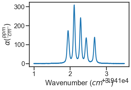
spec_1 = MATS.simulate_spectrum(PARAM_LINELIST, wave_min, wave_max, wave_step,
temperature = 25, pressure = 100, molefraction = { 100 :1e-9},
isotope_list = HITRAN_Hg_isolist, natural_abundance = True, SNR = 1000, filename = '100 Torr',)
spec_2 = MATS.simulate_spectrum(PARAM_LINELIST, wave_min, wave_max, wave_step,
temperature = 25, pressure = 500, molefraction = { 100 :1e-9},
isotope_list = HITRAN_Hg_isolist, natural_abundance = True, SNR = 1000,filename = '500 Torr',)
spec_1.plot_wave_alpha()
spec_2.plot_wave_alpha()

Construct Dataset and Generate Fit Parameters
The construction of the dataset and the generate fit parameter classes act as normal. For the generation of the fit parameter line list, the example below shows how the vary_variable input dictionaries function with multiple isotopes. Specifically, in the example below the VP is used as the fitting line shape, where the spectra were simulated with the SDVP. All parameters are constrained across the spectra and the only parameters being floated are the collisional broadening terms for all isotopes.
SPECTRA = MATS.Dataset([spec_1, spec_2], 'Mercury Fitting',PARAM_LINELIST )

#Generate Baseline Parameter list based on number of etalons in spectra definitions and baseline order
BASE_LINELIST = SPECTRA.generate_baseline_paramlist()


FITPARAMS = Generate_FitParam_File(SPECTRA, PARAM_LINELIST, BASE_LINELIST, lineprofile = 'VP', linemixing = False,
                               fit_intensity = Fit_Intensity, threshold_intensity = IntensityThreshold, sim_window = wave_range,
                               nu_constrain = True, sw_constrain = True, gamma0_constrain = True, delta0_constrain = True,
                                aw_constrain = True, as_constrain = True,
                                nuVC_constrain = True, eta_constrain =True, linemixing_constrain = True,
                               additional_columns = ['trans_id'])

FITPARAMS.generate_fit_param_linelist_from_linelist(vary_nu = {100:{1:False, 2:False, 3:False, 4: False, 5:False, 6:False, 7:False, 8:False, 9:False, 10: False}},
                                                 vary_sw ={100:{1:False, 2:False, 3:False, 4: False, 5:False, 6:False, 7:False, 8:False, 9:False, 10: False}},
                                                 vary_gamma0 = {100:{1:True, 2:True, 3:True, 4: True, 5:True, 6:True, 7:True, 8:True, 9:True, 10: True}},
                                                 vary_delta0 = {100:{1:False, 2:False, 3:False, 4: False, 5:False, 6:False, 7:False, 8:False, 9:False, 10: False}},
                                                 vary_aw = {100:{1:False, 2:False, 3:False, 4: False, 5:False, 6:False, 7:False, 8:False, 9:False, 10: False}},
                                                 vary_as = {100:{1:False, 2:False, 3:False, 4: False, 5:False, 6:False, 7:False, 8:False, 9:False, 10: False}},
                                                 vary_nuVC = {100:{1:False, 2:False, 3:False, 4: False, 5:False, 6:False, 7:False, 8:False, 9:False, 10: False}},
                                                 vary_eta = {100:{1:False, 2:False, 3:False, 4: False, 5:False, 6:False, 7:False, 8:False, 9:False, 10: False}},
                                                 vary_linemixing = {100:{1:False, 2:False, 3:False, 4: False, 5:False, 6:False, 7:False, 8:False, 9:False, 10: False}})

FITPARAMS.generate_fit_baseline_linelist(vary_baseline = False, vary_molefraction = {100: False}, vary_xshift = False,
                                   vary_etalon_amp= False, vary_etalon_period= False, vary_etalon_phase= False)
Fit Spectra
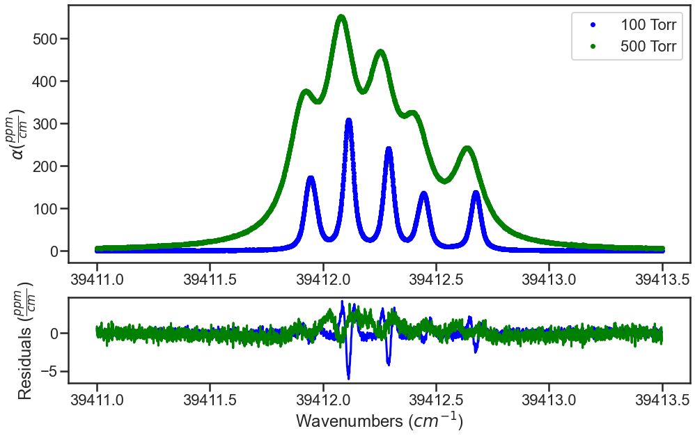
Fitting follows the same strucutre described in Fitting Experimental Spectra. The fit results shown below are the result of fitting spectra simulated with the SDVP with the VP and only allowing the collsional broadening terms to float. The residuals at both pressures show the expected w-shaped residuals.
fit_data = MATS.Fit_DataSet(SPECTRA,'Baseline_LineList', 'Parameter_LineList', minimum_parameter_fit_intensity = Fit_Intensity, weight_spectra = False)
params = fit_data.generate_params()
result = fit_data.fit_data(params, wing_cutoff = 25)
fit_data.residual_analysis(result, indv_resid_plot=False)
fit_data.update_params(result)
SPECTRA.generate_summary_file(save_file = True)
SPECTRA.plot_model_residuals()
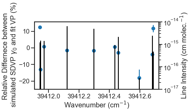
We can compare the VP fit collisional broadening fit results to the SDVP collisional broadening values used in the simulation. On the secondary y-axis is a stem plot showing the line intensity for the lines. This highlights that the lines that deviated the most from the simulated collisional broadening value were weaker and/or closely spaced to other isotope transitions.
Parameter_Linelist= pd.read_csv('Parameter_Linelist.csv', index_col = 0)
simulated_gamma0_air = PARAM_LINELIST['gamma0_air'].values[0]

fig, ax1 = plt.subplots(constrained_layout=True, figsize= [9, 4.5])
ax2 = ax1.twinx()
ax2.stem(Parameter_Linelist['nu'].values,Parameter_Linelist['sw'].values*Parameter_Linelist['sw_scale_factor'].values, "k", markerfmt = 'None', basefmt = 'None')
ax1.errorbar(Parameter_Linelist['nu'].values, 100*(Parameter_Linelist['gamma0_air'].values - simulated_gamma0_air)/ simulated_gamma0_air,
          yerr = 100*(Parameter_Linelist['gamma0_air_err'].values)/ Parameter_Linelist['gamma0_air'].values,fmt = "o")


ax2.set_ylim(1e-17, 1e-14)
ax1.ticklabel_format(axis = 'x', useOffset = False)
ax2.set_yscale('log')
ax1.set_xlabel('Wavenumber (cm$^{-1}$)')
ax2.set_ylabel('Line Intensity (cm molec.$^{-1}$)')
ax1.set_ylabel('Relative Differnece between \n simulated SDVP $\\gamma_{0}$ and fit VP (%)')