|
HTGS
v2.0
The Hybrid Task Graph Scheduler
|
|
HTGS
v2.0
The Hybrid Task Graph Scheduler
|
In this tutorial we revisit Tutorial 3A to investigate performance through the HTGS profiling/debugging visualization. One powerful component of HTGS is its high level abstractions that is explicitly represented throughout the analysis and implementation. These abstractions persist throughout execution, which can be used to profile and identify bottlenecks at a high level of abstraction.
This tutorial uses the same implementation, data, tasks, and dependencies as presented in Tutorial 3A Data.
Building a htgs::TaskGraphConf will create an explicit represenatation of the task graph, which can be visualized using htgs::TaskGraphConf::writeDotToFile. This function can be called before or after launching the graph using the htgs::TaskGraphRuntime.
There are nine flags that are specified in the <htgs/types/TaskGraphDotGenFlags.hpp> header file, which can be used to configure the output of the visualization.
When profiling a htgs::TaskGraphConf, it is best to call htgs::TaskGraphConf::writeDotToFile after a call to htgs::TaskGraphRuntime::waitForRuntime. This ensures that the graph has finished executing.
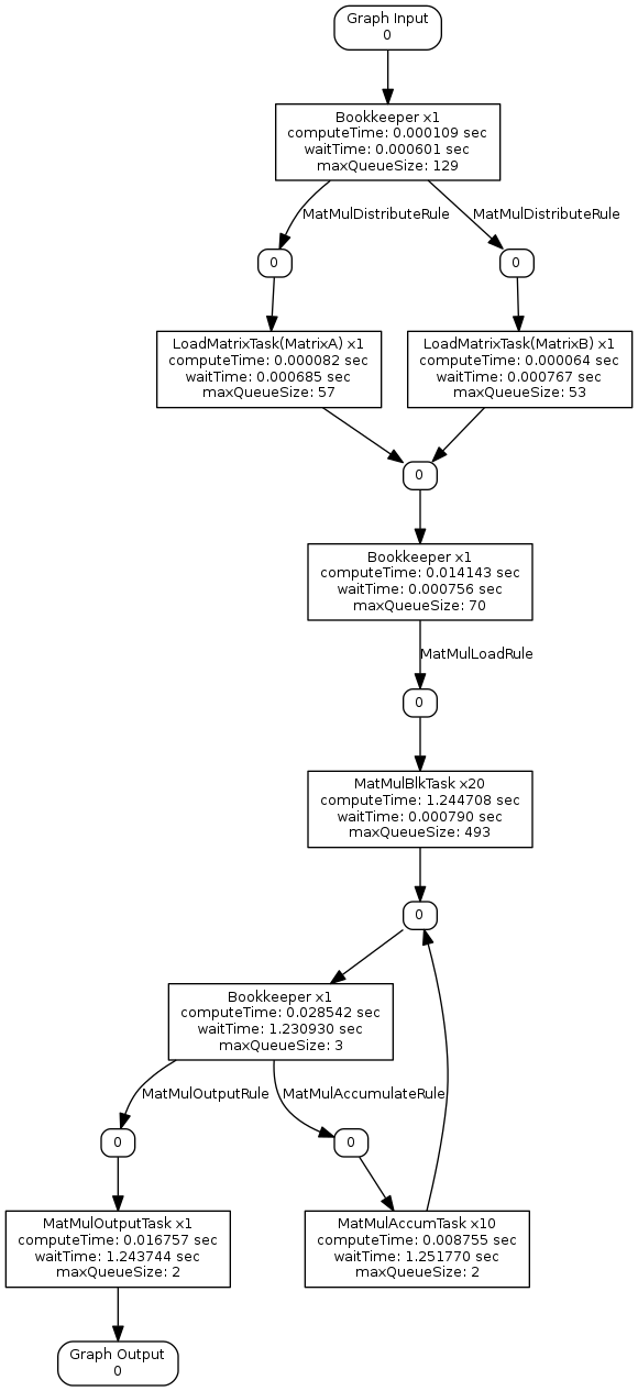
Below are examples of visualizing the htgs::TaskGraphConf from Tutorial3A before and after executing the graph.
The graphs above were converted to a png (or pdf with -Tpdf) file using the following commands:
In the figures above, each graph shows the explicit representation that is to be used to process matrix multiplication. Tasks have the "x<#>" notation, where <#> represents the number of tasks copied and bound to separate threads. These threads have not been spawned yet, but provide an indicator as to how many threads will be spawned to execute each task within the graph. Every htgs::Bookkeeper have annotated output edges that provide the name of the rule that is responsible for processing that edge.
In addition there are nodes between tasks that represent the htgs::Connector, which manages the thread-safe queue for the task. The number within this node represents the number of active connections that will be producing data for the connector. During execution, if this number reaches zero, then that edge is considered no longer receiving data (terminated), which can be checked with htgs::Connector::isInputTerminated. At the top and bottom of the visualization are the "Graph Input" and "Graph Output" nodes, which represent the input and output connectors for the htgs::TaskGraphConf.
In the in-out-graph.png figure, every task have additional details showing the specific input and output data types for each task.
These figures can be used to ensure the graph representation that is done during analysis maps well into the actual implementation.
During compilation we include "-DPROFILE" to enable profiling of the graph.
We execute this version using the following command (includes associated output):
The code above will generate five visualizations. (with adding -DPROFILE to compilation)
As shown in the source code above, each DOTGEN flag can be aggregated using the bit-wise OR operator.
Below are the resulting figures for each graph after using the following commands:
color-compute-time-profile-graph.png
color-wait-time-profile-graph.png
color-max-q-sz-profile-graph.png
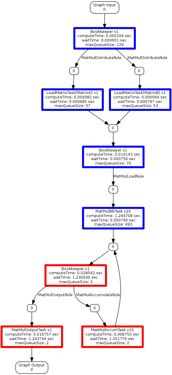
profile-graph.png shows the compute time, wait time, and max queue size for each task. Any task that has multiple threads associated are reporting the average timings for that task.
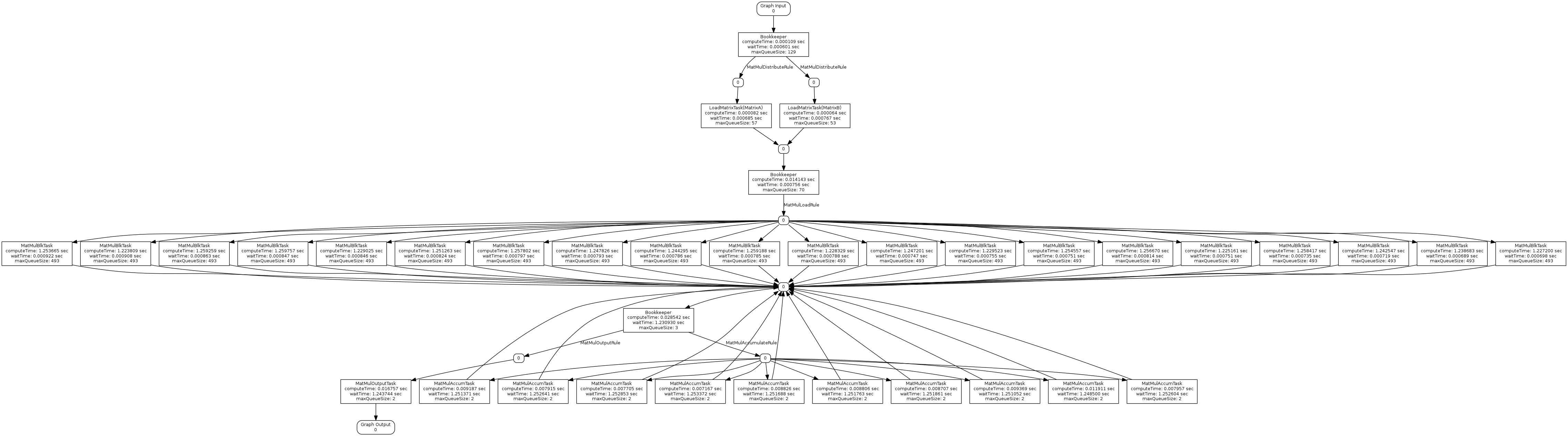
profile-all-threads-graph.png shows the fully expanded graph and all threading.
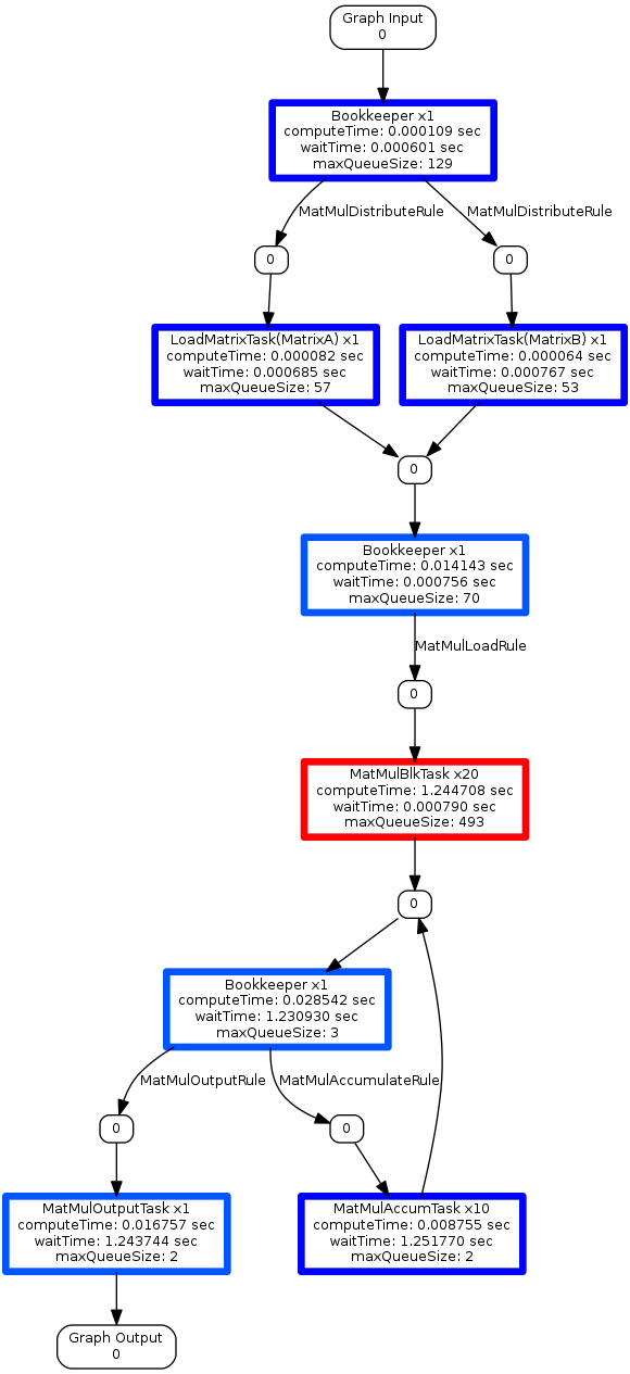
These graphs are useful to get a glimpse at the overall timings for each task. Using the coloring options provides a much clearer picture to pinpoint the bottleneck(s) within an implementation. First, the color-compute-time-profile-graph.png creates a color map based around the compute times. The cooler blue times are less impactful, whereas the hot red times have high impact. The MatMulBlkTask is colored bright red, which indicates this task is the main bottleneck. The color-wait-time and color-max-q-sz graphs support this observation. In addition, the color-wait-time and color-max-q-sz are showing that the MatMulAccumTask and MatMulOutPutTaskWithDisk tasks are spending the majority of their time waiting for data. Improving the execution time of the MatMulBlkTask should reduce reduce the wait time for these tasks; however, in some cases modifying traversal patterns for inserting data into the htgs::TaskGraphConf from the main thread or optimizing data locality can provide additional benefits.
To improve the performance of this implementation, we investigate methods for improving the MatMulBlkTask.
The MatMulBlkTask can be thought of as an in-core computational kernel that executes on the CPU. Methods for fine-grained parallelism, such as utilizing L1 cache and instruction-level parallelism can be used to improve the overall CPU utilization for this task. Alternatively, an accelerator could be incorporated into the graph to offload the computation to high bandwidth massively parallel hardware (shown in Tutorial4A).
The current implementation of matrix multiplication uses a triple nested for loop that iterates across the entire matrix, shown here. Instead of taking the time to optimize this code, existing in-core compute kernels are available, such as those from OpenBLAS. OpenBLAS implements various basic linear algebra operators and will generate a per-architecture optimized library. Using this library should boost the performance for our MatMulBlkTask.
Before incorporating OpenBLAS into the MatMulBlkTask, one additional component can be taken into account to quantify this improvement.
Each htgs::ITask contain two additional functions that will add customizable details to the visualization. This can be applied before or after execution of an htgs::TaskGraphConf.
Implementing the htgs::ITask::debugDotNode is intended to add debug output. The htgs::ITask::getDotCustomProfile can be used to provide additional custom profiling data that will be added to the dot visualization. This can be used in conjunction with htgs::ITask::getComputeTime, to obtain the compute time of the htgs:ITask in microseconds.
Below, we incorporate a GFLops benchmark into the MatMulBlkTask. This allows us to track the performance within this task.
Using the above implementation of the task outputs the number of gflops performed by a task.
Using this variant, we execute with the following command and output the task graph dot file.
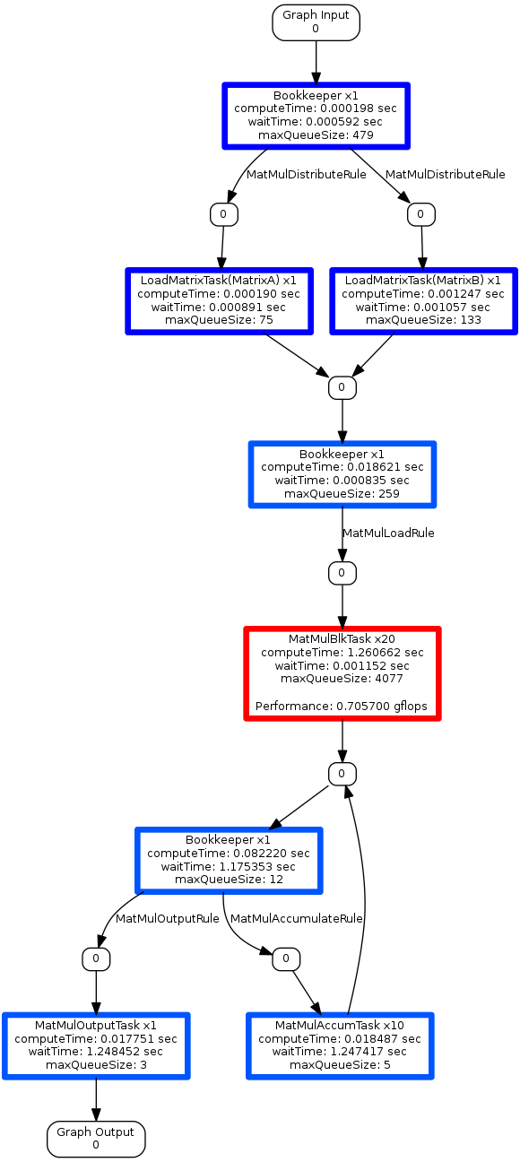
This implementation achieves 13.5 GFlops. Viewing the graph visualization, we see the first thread for the MatMulBlkTask is achieving 0.7 GFlops. With 20 threads this is approximately 14 GFlops, note that this is not taking into account the final accumulation step. To view the actual GFlop rating for each MatMulBlkTask thread, we can use the DOTGEN_FLAG_SHOW_ALL_THREADING flag, also shown below.
Profile with all threads and GFlops
Now that we have a clear metric to base our task performance off of, we incorporate OpenBLAS into the computation.
Example call for OpenBLAS, also found here:
To enable using OpenBLAS in the HTGS-Tutorials, define the following during cmake (or cmake-gui/ccmake)
Defining these options will enable using OpenBLAS for Tutorial 3. We execute the same command as above with OpenBLAS enabled.
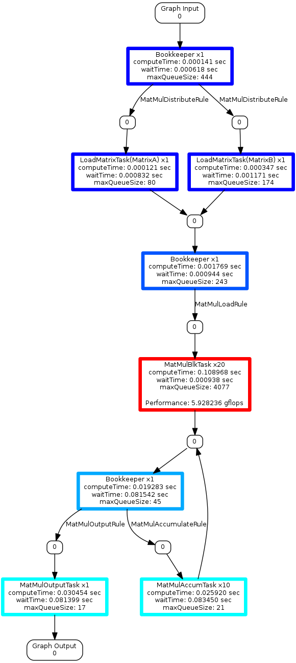
With OpenBLAS enabled, the implementation now achieves 148.1 GFlops. The graph visualization now shows the first thread achieves 5.92 Gflops, which is approximately, 118.4 GFlops. Viewing all of the threads shows a clearer picture about utilization, where some threads achieved up to 12.79 GFlops.
Profile with all threads OpenBLAS
Overall, this shows an overall speedup of 10x for this small problem size.
Now that the MatMulBlk task has been improved, we can experiment further to analyze the impact of block-size. I leave this task up to you to see how far you can push the GFlops performance for the MatMulBlk task by altering the matrix dimensions and block sizes.
In this tutorial, we revisited the matrix multiplication implementation from Tutorial3A.
Working at a higher level abstractions within HTGS enables analyzing the algorithm at that abstraction, which can be used to identify bottlenecks and make decisions on a per-task basis. More advanced techniques, such as changing data representations and traversal patterns can also be used to improve utilization and data reuse.
An implementation that adds memory mapped files and the disk are also available in the HTGS-Tutorials code-base. Memory mapped files will only work on Linux and OSX systems. Next, Tutorial4 will revisit matrix multiplication and incorporate NVIDIA GPUs into the computation. If you do not have an NVIDIA GPU, then skip to Tutorial6.
 1.8.13
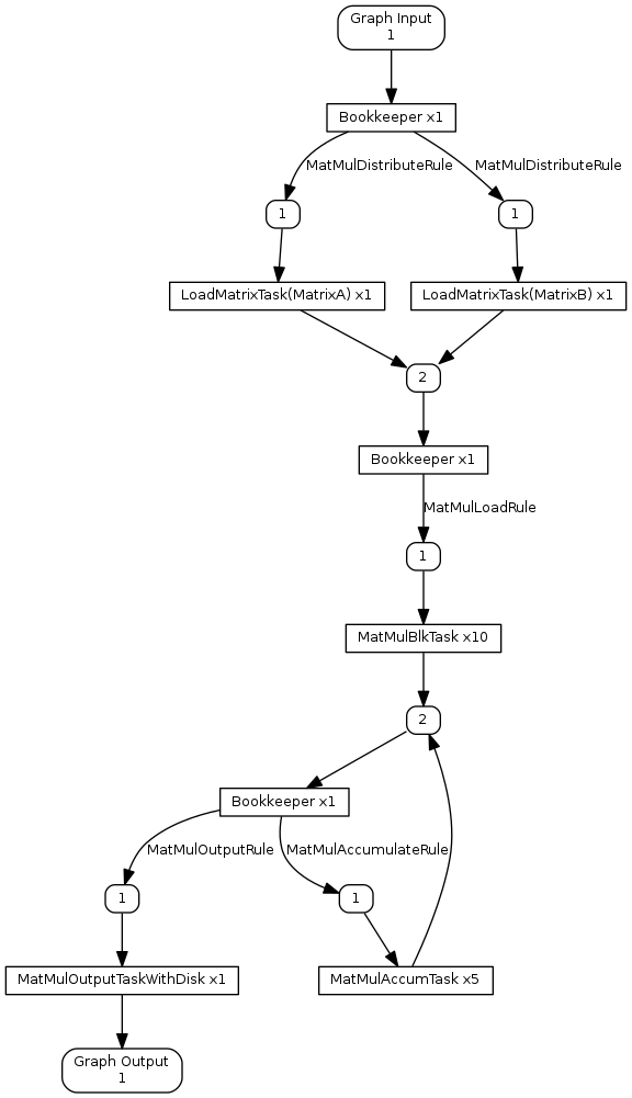