Performance¶

When datasets become increasingly large, the number of unique thresholds can grow significantly. To maximize performance, we rely on numpy's "broadcasting" feature to perform operations using its C-backend, rather than Python.

Vectorize & Memoize¶

Because looping in python is slow, we rely on boolean matrix operations to calculate the contingency counts. At the core of Contingent.from_scalar is a call to numpy.less_equal.outer, which broadcasts the thresholding operation over all possible levels simultaneously.

This is reasonably fast, able to calculate e.g. APS only marginally slower than the scikit-learn implementation. In addition, the one-time calculation of the "full" contingency set has the added benefit of amortizing the cost of subsequent metric calculations significantly.

Let's make a much larger test case than before, by adding white noise to a known ground-truth.

rng = np.random.default_rng(24) # (1)! 
y_src = rng.random(1000)
y_true = y_src>0.7

y_pred = y_src + 0.05*rng.normal(size=1000)

1. Did you know? 24mph is the cruising airspeed velocity of an unladen (european) swallow

from sklearn.metrics import average_precision_score, matthews_corrcoef
%timeit average_precision_score(y_true, y_pred)
%timeit Contingent.from_scalar(y_true, y_pred).expected('aps')

Mbig = Contingent.from_scalar(y_true, y_pred)
%timeit Mbig.expected('aps')

1.07 ms ± 231 μs per loop (mean ± std. dev. of 7 runs, 1,000 loops each)
2.83 ms ± 55.4 μs per loop (mean ± std. dev. of 7 runs, 100 loops each)
30.3 μs ± 341 ns per loop (mean ± std. dev. of 7 runs, 10,000 loops each)

This means that, with a single Contingent object, all of the various metrics can be calculated from then on in mere microseconds.

And when scikit-learn does not have optimized aggregation functions, Contingent can continue on just as well. Say you wish to find the expected value of the MCC score over all thresholds; using a Contingent object results in an order of magnitude speed increase.

%timeit np.mean([matthews_corrcoef(y_true,x) for x in Mbig.y_pred])
%timeit M1000.expected('mcc')

1.36 s ± 576 ms per loop (mean ± std. dev. of 7 runs, 1 loop each)
176 μs ± 10.9 μs per loop (mean ± std. dev. of 7 runs, 10,000 loops each)

Subsampling Approximation¶

The limit to this amortization comes from your RAM: the outer-product matrix we use to vectorize contingency counting can get huge.

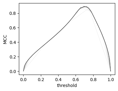
To mitigate this, Contingent.from_scalar has a subsamples option which allows you to approximate the threshold values with an interpolated subset distributed according to the originals.

With only a few subsamples, the score curves quickly converge to their "true" values.

# rng.normal(
plt.figure(figsize=(4,3))
for subs in (5,10,15, 20, 25, 30,50,75,100): 
    plt.plot(
        np.linspace(0,1,subs),
        (Contingent.from_scalar(y_true, y_pred, subsamples=subs)).mcc,
        lw=0.5, color=f'{1-subs/100:.1f}'
    )
plt.ylabel('MCC')
plt.xlabel('threshold');

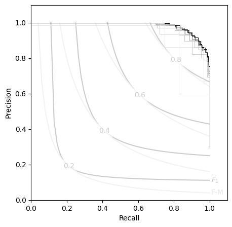
Likewise, the P-R curves:

plt.figure(figsize=(5,5))
PR_contour()

for subs in (5,10,15, 20, 25, 30,50,75,100): 
    Msubs = Contingent.from_scalar(y_true, y_pred, subsamples=subs)
    plt.step(Msubs.recall, Msubs.precision, lw=0.7, color=f'{1-subs/100:.1f}', where='post')

This allows Contingent objects to handle some quite large datasets:

y_src = rng.random(int(1e6))
y_true = y_src>0.7

y_pred = y_src + 0.05*rng.normal(size=int(1e6))
# from sklearn.metrics import average_precision_score, matthews_corrcoef
%timeit average_precision_score(y_true, y_pred)
%timeit Contingent.from_scalar(y_true, y_pred, subsamples=200)

M200 = Contingent.from_scalar(y_true, y_pred, subsamples=200)

%timeit M200.expected('aps')

511 ms ± 21 ms per loop (mean ± std. dev. of 7 runs, 1 loop each)
678 ms ± 203 ms per loop (mean ± std. dev. of 7 runs, 1 loop each)
28 μs ± 411 ns per loop (mean ± std. dev. of 7 runs, 10,000 loops each)

print(
    '{:.4g}'.format(average_precision_score(y_true, y_pred)), 
    '{:.4g}'.format(M200.expected('aps'))
)

0.9865 0.9858