Using Prefabricated Pipelines#

[1]:

%load_ext autoreload
%autoreload 2

[2]:

# Import required libraries
import matplotlib.pyplot as plt
import numpy as np
from AFL.double_agent import *
from AFL.double_agent.data import example_dataset1
from AFL.double_agent.prefab import load_prefab, list_prefabs, combine_prefabs

Introduction#

Prefabricated pipelines (prefabs) are pre-configured pipelines that can be easily loaded and used in your projects. This tutorial will guide you through the process of loading and using prefabricated pipelines from the AFL.double_agent.prefab module.

Prefabricated pipelines are particularly useful when:

You have common processing steps that you use frequently
You want to share pipeline configurations with colleagues
You want to create building blocks that can be combined into more complex pipelines

In this tutorial, we’ll:

Load an example dataset
Load a prefabricated pipeline
Inspect the pipeline
Customize the pipeline to work with our dataset
Execute the pipeline and analyze the results

Let’s get started!

Google Colab Setup#

Only uncomment and run the next cell if you are running this notebook in Google Colab or if don’t already have the AFL-agent package installed.

[3]:

# !pip install git+https://github.com/usnistgov/AFL-agent.git

Listing Available Prefabs#

Next, let’s check what prefabricated pipelines are available:

[5]:

# List all available prefabricated pipelines with descriptions
list_prefabs()


Available Prefabricated Pipelines:
|-----------------------|-------------------------------------------------------------------------------------------------------------|
| Name                  | Description                                                                                                 |
|-----------------------|-------------------------------------------------------------------------------------------------------------|
| find_boundaries       | A simlarity-clustering-classification pipeline for finding boundaries in measurement data                   |
| preprocess            | A pipeline that generates a Cartesian grid, normalizes data, and calculates derivatives using Savgol filter |
| similarity_clustering | A simlarity-clustering pipeline for clustering measurements into groups                                     |
|-----------------------|-------------------------------------------------------------------------------------------------------------|
Total: 3 prefabricated pipeline(s)

Loading a Prefabricated Pipeline#

Let’s load a prefabricated pipeline called “preprocess”:

[6]:

# Load the "preprocess" prefabricated pipeline
pipeline = load_prefab("preprocess")
pipeline.print()

PipelineOp                               input_variable ---> output_variable
----------                               -----------------------------------
0  ) <CartesianGridGenerator>            CartesianGridGenerator ---> composition_grid
1  ) <Standardize>                       composition_grid ---> normalized_composition_grid
2  ) <Standardize>                       composition ---> normalized_composition
3  ) <SavgolFilter>                      measurement ---> measurement_derivative0
4  ) <SavgolFilter>                      measurement ---> measurement_derivative1
5  ) <SavgolFilter>                      measurement ---> measurement_derivative2

Input Variables
---------------
0) CartesianGridGenerator
1) composition
2) measurement

Output Variables
----------------
0) normalized_composition_grid
1) normalized_composition
2) measurement_derivative0
3) measurement_derivative1
4) measurement_derivative2

Inspecting the Pipeline Structure#

To better understand the pipeline we’ve loaded, we can visualize it using the .draw() method:

[7]:

# Visualize the pipeline structure
pipeline.draw();

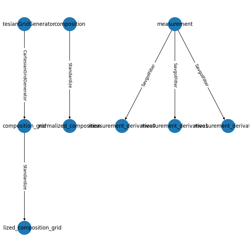
../_images/tutorials_using_prefab_13_0.png

Generating Code for the Pipeline#

The print_code() method allows us to extract Python code that recreates the pipeline. This is particularly useful when we want to:

Understand how the pipeline was built
Modify the pipeline to suit our needs
Create a new pipeline based on the existing one

Now, let’s reproduce the code from the Pipeline and modify it to work with our example dataset. You’ll need to make the following changes:

Change the dim argument for the Savgol filters from “q” to “x” to match the example_dataset

[29]:

# Generate code for the pipeline
pipeline.print_code()

Pipeline code has been prepared in a new cell below.

[34]:

with Pipeline(name = "preprocess") as p:
    CartesianGrid(
        output_variable="composition_grid",
        grid_spec={'A': {'min': 0.0, 'max': 10.0, 'steps': 50}, 'B': {'min': 0.0, 'max': 25.0, 'steps': 50}},
        sample_dim="grid",
        component_dim="component",
        name="CartesianGridGenerator",
    )

    Standardize(
        input_variable="composition_grid",
        output_variable="normalized_composition_grid",
        dim="grid",
        component_dim="component",
        scale_variable=None,
        min_val={'A': 0.0, 'B': 0.0},
        max_val={'A': 10.0, 'B': 25.0},
        name="Standardize",
    )

    Standardize(
        input_variable="composition",
        output_variable="normalized_composition",
        dim="sample",
        component_dim="component",
        scale_variable=None,
        min_val={'A': 0.0, 'B': 0.0},
        max_val={'A': 10.0, 'B': 25.0},
        name="Standardize",
    )

    SavgolFilter(
        input_variable="measurement",
        output_variable="measurement_derivative0",
        dim="x",
        xlo=None,
        xhi=None,
        xlo_isel=None,
        xhi_isel=None,
        pedestal=None,
        npts=250,
        derivative=0,
        window_length=31,
        polyorder=2,
        apply_log_scale=True,
        name="SavgolFilter",
    )

    SavgolFilter(
        input_variable="measurement",
        output_variable="measurement_derivative1",
        dim="x",
        xlo=None,
        xhi=None,
        xlo_isel=None,
        xhi_isel=None,
        pedestal=None,
        npts=250,
        derivative=1,
        window_length=31,
        polyorder=2,
        apply_log_scale=True,
        name="SavgolFilter",
    )

    SavgolFilter(
        input_variable="measurement",
        output_variable="measurement_derivative2",
        dim="x",
        xlo=None,
        xhi=None,
        xlo_isel=None,
        xhi_isel=None,
        pedestal=None,
        npts=250,
        derivative=2,
        window_length=31,
        polyorder=2,
        apply_log_scale=True,
        name="SavgolFilter",
    )

Visualizing the Results#

Let’s visualize the results of our pipeline:

[40]:

fig,axes = plt.subplots(1,2,figsize=(8,3))
result.composition.to_dataset('component').plot.scatter(x='A',y='B',ax=axes[0])
result.normalized_composition.to_dataset('component').plot.scatter(x='A',y='B',ax=axes[1])

[40]:

<matplotlib.collections.PathCollection at 0x3135b9450>

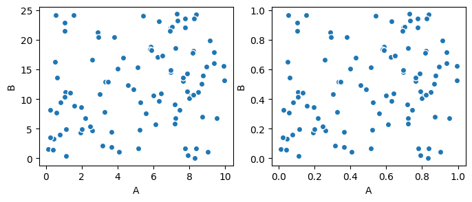
../_images/tutorials_using_prefab_20_1.png

We can see that the relative positions of the compositions are unchanged, we simply renormalized the bounds of the data.

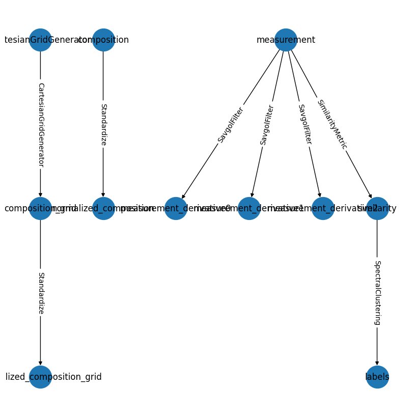
Combining Multiple Prefabs#

One of the powerful features of prefabricated pipelines is the ability to combine multiple prefabs into a single pipeline:

[44]:

# Combine multiple prefabs if you have more than one available
combined_pipeline = combine_prefabs(["preprocess", "similarity_clustering"], new_name="CombinedPipeline")
combined_pipeline.draw();

../_images/tutorials_using_prefab_23_0.png

Conclusion#

In this tutorial, we learned how to:

Load an example dataset from the AFL.double_agent.data module
List and load prefabricated pipelines from the AFL.double_agent.prefab module
Inspect the structure of a pipeline using .draw() and .print() methods
Generate and modify code for a pipeline using .print_code()
Run a customized pipeline on a dataset and visualize the results
Combine multiple prefabricated pipelines

Prefabricated pipelines provide a convenient way to reuse and share pipeline configurations, making your analysis workflows more efficient and reproducible.