Advanced cubic mixing rules

In the advanced cubic mixing rules, the conventional cubic EOS is taken as the basis for the method (usually Peng-Robinson), but different rules are used for the attractive term $a_m$. The formulation reads:

$$\frac{a_m}{b_m}=\sum _i{z}_i\frac{a_i}{b_i}+\frac{a_{\mathrm{r}\mathrm{e}\mathrm{s}}^{E,\gamma }}{CEoS}$$

where $CEoS$ is a scaling parameter that is in principle linked with the EOS coefficients, but can also be allowed to be an adjustable parameter. The $a_i$ and $b_i$ are the pure fluid values of component $i$. The $z_i$ are mole fractions. The mixture covolume is given by

$$b_m=\sum _i\sum _j{z}_i{z}_j{b}_{ij}$$

with

$$b_{ij}={\left(\frac{b_i^{1/s}+b_j^{1/s}}{2}\right)}^s$$

The heart of the method is the definition of $a_{\mathrm{r}\mathrm{e}\mathrm{s}}^{E,\gamma }$, the residual contribution (not in the conventional thermodynamic sense) to the excess Helmholtz energy. There are many possible models here, but one that seems to work well is that of Wilson, for which the expression reads:

$$\frac{a_{\mathrm{r}\mathrm{e}\mathrm{s}}^{E,\gamma }}{RT}=-\sum _i{z}_i\ln (\sum _j{z}_j{\mathrm{\Omega }}_{ji}(T))-\sum _i{z}_i\ln \left(\frac{{\varphi }_i}{z_i}\right)$$

with

$${\mathrm{\Omega }}_{ji}=\frac{v_j}{v_i}\exp (-A_{ij}/T)$$

and

$$\frac{{\varphi }_i}{z_i}=\frac{v_i}{\sum _k{z}_k{v}_k}$$

with the $v_i=b_i$. The parameter $A_{ij}\ne A_{ji}$ in general, and is also given temperature dependence, which is also not supposed to be present according to the derivation. Thus, the models for $A_{ij}$ read something like this here:

$$A_{ij}=m_{ij}T+n_{ij}$$

so $m_{ij}$ is non-dimensional and $n_{ij}$ has units of temperature because $A_{ij}$ has units of temperature.

import numpy, matplotlib.pyplot as plt, numpy as np, pandas
import teqp
teqp.__version__

'0.22.0'

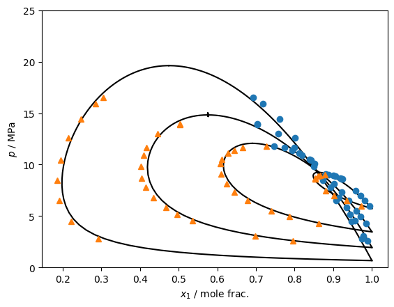
# Four isotherms of experimental data from doi: 10.1016/j.fluid.2016.05.015
import io, pandas
dat = pandas.read_csv(io.StringIO("""PointID y1 uy1 x1 ux1 p/bar up T/K
1 0.0274 0.0007 0.0068 0.0002 59.830 0.053 293.10
2 0.0664 0.0014 0.0183 0.0004 64.864 0.080 293.10
3 0.0978 0.0020 0.0298 0.0007 69.772 0.080 293.10
4 0.1199 0.0024 0.0424 0.0009 74.737 0.080 293.10
5 0.1219 0.0028 0.1132 0.0023 89.869 0.080 293.10
6 0.1339 0.0024 0.0995 0.0022 89.198 0.080 293.10
7 0.1399 0.0026 0.0943 0.0020 88.853 0.080 293.10
8 0.1461 0.0027 0.0823 0.0019 86.962 0.080 293.10
9 0.1466 0.0028 0.0778 0.0017 85.942 0.080 293.10
10 0.1466 0.0028 0.0772 0.0016 85.868 0.080 293.10
1 0.1378 0.0027 0.0159 0.0004 42.667 0.051 273.08
2 0.2143 0.0038 0.0297 0.0007 49.547 0.051 273.08
3 0.2612 0.0043 0.0411 0.0009 55.238 0.051 273.08
4 0.3209 0.0049 0.0609 0.0013 65.069 0.088 273.08
5 0.3554 0.0051 0.0786 0.0016 73.395 0.088 273.08
6 0.3758 0.0052 0.0978 0.0019 81.061 0.088 273.08
7 0.3903 0.0053 0.1190 0.0023 90.706 0.088 273.08
8 0.3914 0.0053 0.1477 0.0028 100.966 0.088 273.08
9 0.3879 0.0053 0.1614 0.0030 104.806 0.088 273.08
10 0.3724 0.0052 0.1875 0.0033 110.846 0.088 273.08
11 0.3550 0.0051 0.2068 0.0036 114.105 0.088 273.08
12 0.2727 0.0044 0.2531 0.0041 118.020 0.088 273.08
13 0.3343 0.0049 0.2268 0.0038 116.295 0.088 273.08
1 0.2048 0.0038 0.0106 0.0003 25.754 0.050 253.05
2 0.3019 0.0049 0.0217 0.0005 30.479 0.050 253.05
3 0.4638 0.0056 0.0436 0.0010 45.352 0.050 253.05
4 0.5319 0.0056 0.0647 0.0014 58.188 0.050 253.05
5 0.5854 0.0054 0.1077 0.0021 78.315 0.084 253.05
6 0.5979 0.0054 0.1497 0.0028 98.276 0.084 253.05
7 0.5898 0.0054 0.1801 0.0032 109.241 0.084 253.05
8 0.5042 0.0057 0.0570 0.0012 51.343 0.084 253.05
9 0.5644 0.0055 0.0861 0.0017 67.594 0.084 253.05
10 0.5949 0.0054 0.1267 0.0024 86.883 0.084 253.05
11 0.5826 0.0054 0.2015 0.0035 116.614 0.084 253.05
12 0.5537 0.0055 0.2431 0.0040 129.873 0.084 253.05
13 0.4973 0.0055 0.2971 0.0046 139.161 0.084 253.05
14 0.4971 0.0055 0.2972 0.0046 139.261 0.084 253.05
1 0.7076 0.0050 0.0257 0.0006 27.983 0.056 223.10
2 0.7774 0.0041 0.0522 0.0011 44.918 0.056 223.10
3 0.8077 0.0036 0.0930 0.0019 64.906 0.081 223.10
4 0.8131 0.0035 0.1261 0.0024 84.799 0.081 223.10
5 0.8057 0.0035 0.1584 0.0029 104.410 0.081 223.10
6 0.7843 0.0038 0.1982 0.0035 125.782 0.081 223.10
7 0.7533 0.0041 0.2380 0.0040 144.287 0.081 223.10
8 0.7150 0.0045 0.2813 0.0044 159.015 0.081 223.10
9 0.6942 0.0047 0.3064 0.0047 165.347 0.081 223.10
"""), sep='\s+', engine='python')

# Model from Lasala, FPE, 2016: https://doi.org/10.1016/j.fluid.2016.05.015
j = {
    "kind": "advancedPRaEres",
    "model": {
       "Tcrit / K": [304.21, 126.19],
       "pcrit / Pa": [7.383e6, 3395800.0],
       "alphas": [{"type": "PR78", "acentric": 0.22394}, {"type": "PR78", "acentric": 0.0372}],
       "aresmodel": {"type": "Wilson", "m": [[0.0, -3.4768], [3.5332, 0.0]], "n": [[0.0, 825], [-585, 0.0]]},
       "options": {"s": 2.0, "brule": "Quadratic", "CEoS": -0.52398}
    }
}

model = teqp.make_model(j)
for T in [223.15, 253.05, 273.08, 293.1]:
    ipure = 0

    [rhoL0, rhoV0] = model.superanc_rhoLV(T, ipure)

    rhovecL0 = np.array([0.0, 0.0]); rhovecL0[ipure] = rhoL0
    rhovecV0 = np.array([0.0, 0.0]); rhovecV0[ipure] = rhoV0

    J = model.trace_VLE_isotherm_binary(T, rhovecL0, rhovecV0)
    df = pandas.DataFrame(J)
    plt.plot(df['xL_0 / mole frac.'], df['pL / Pa']/1e6,'k')
    plt.plot(df['xV_0 / mole frac.'], df['pV / Pa']/1e6,'k')

plt.plot(1-dat['x1'], dat['p/bar']/10, 'o')
plt.plot(1-dat['y1'], dat['p/bar']/10, '^')

plt.gca().set(xlabel='$x_1$ / mole frac.', ylabel='$p$ / MPa', ylim=(0, 25))
plt.show()