PC-SAFT¶

The PC-SAFT implementation in teqp is based on the implementation of Gross and Sadowski (https://doi.org/10.1021/ie0003887), with the typo from their paper fixed. It does NOT include the association contribution, only the dispersive contributions.

The model in teqp requires the user to specify the values of sigma, epsilon/kB, and m for each substance. A very few substances are hardcoded in teqp, for testing purposes.

The Python class is here: PCSAFTEOS

[1]:

import teqp
import numpy as np
teqp.__version__

[1]:

'0.22.0'

[2]:

TeXkey = 'Gross-IECR-2001'
ms = [1.0, 1.6069, 2.0020]
eoverk = [150.03, 191.42, 208.11]
sigmas = [3.7039, 3.5206, 3.6184]

coeffs = []
for i in range(len(ms)):
    c = teqp.SAFTCoeffs()
    c.m = ms[i]
    c.epsilon_over_k = eoverk[i]
    c.sigma_Angstrom = sigmas[i]
    coeffs.append(c)

model = teqp.PCSAFTEOS(coeffs)

[3]:

# Here are some rudimentary timing results
T = 300.0
rhovec = np.array([3.0, 4.0, 5.0])
rho = rhovec.sum()
x = rhovec/np.sum(rhovec)
%timeit model.get_fugacity_coefficients(T,rhovec)
%timeit (-1.0)*model.get_Ar20(T, rho, x)
%timeit model.get_partial_molar_volumes(T, rhovec)

3.56 μs ± 5.29 ns per loop (mean ± std. dev. of 7 runs, 100,000 loops each)
3.86 μs ± 13.3 ns per loop (mean ± std. dev. of 7 runs, 100,000 loops each)
15 μs ± 80 ns per loop (mean ± std. dev. of 7 runs, 100,000 loops each)

The model parameters can be queried:

[4]:

model.get_m(), model.get_epsilon_over_k_K(), model.get_sigma_Angstrom()

[4]:

(array([1.    , 1.6069, 2.002 ]),
 array([150.03, 191.42, 208.11]),
 array([3.7039, 3.5206, 3.6184]))

Adjusting k_ij¶

Fine-tuned values of \(k_{ij}\) can be provided when instantiating the model. A complete matrix of all the \(k_{ij}\) values must be provided. This allows for asymmetric mixing models in which \(k_{ij}\neq k_{ji}\).

[5]:

k_01 = 0.01; k_10 = k_01
kmat = [[0,k_01,0],[k_10,0,0],[0,0,0]]
model = teqp.PCSAFTEOS(coeffs, kmat)

[6]:

# and the matrix of parameters can be printed back out
model.get_kmat()

[6]:

array([[0.  , 0.01, 0.  ],
       [0.01, 0.  , 0.  ],
       [0.  , 0.  , 0.  ]])

Alternative a and b matrices¶

In the PC-SAFT implementation of Gross and Sadowski, they have specified coefficients for the approximations used for the integrals in the perturbation theory (Eqs. A.16 to A.19)

\[I_1 = \sum_{i=0}^6a_i(\bar m)\eta^i\]

\[I_2 = \sum_{i=0}^6b_i(\bar m)\eta^i\]

\[a_i(\bar m) = a_{0i} + \frac{\bar m-1}{\bar m}a_{1i} + \frac{\bar m-1}{\bar m}\frac{\bar m-2}{\bar m}a_{2i}\]

\[b_i(\bar m) = b_{0i} + \frac{\bar m-1}{\bar m}b_{1i} + \frac{\bar m-1}{\bar m}\frac{\bar m-2}{\bar m}b_{2i}\]

and they provide tabulated values in Table 1 in their paper, but other works have identified that some of the limitations of PC-SAFT can be traced back to these universal parameters. Thus, as of version 0.21, two additional options for these parameter matrices are available from the works of Liang et al:

“Liang-IECR-2012”: Approach to Improve Speed of Sound Calculation within PC-SAFT Framework
“Liang-IECR-2014”: New Variant of the Universal Constants in the Perturbed Chain-Statistical Associating Fluid Theory Equation of State

and they can be selected by providing the “ab” field in the JSON data structure. Something like this:

[7]:

spec = {
  "kind": "PCSAFT",
  "model": {
    "names": ["Methane", "Ethane"],
    "ab": "Liang-IECR-2014"
  }
}
teqp.make_model(spec, validate=True)

[7]:

<teqp.teqp.AbstractModel at 0x7ff3a5b35c70>

Superancillary¶

The superancillary equation for PC-SAFT has been developed, and is much more involved than that of the cubic EOS. As a consequence, the superancillary equation has been provided as a separate package rather than integrating it into to teqp to minimize the binary size of teqp. It can be installed from PYPI with: pip install PCSAFTsuperanc

The scaling in the superancillaries uses reduced variables:

\[\tilde T = T/(\epsilon/k_{\rm B})\]

\[\tilde\rho = \rho_{\rm N}\sigma^3\]

where \(\rho_{\rm N}\) is the number density, and the other parameters are from the PC-SAFT model

[8]:

import PCSAFTsuperanc

sigma_m = 3e-10 # [meter]
e_over_k = 150.0 # [K]
m = 5

# The saturation temperature
T = 300

[Ttilde_crit, Ttilde_min] = PCSAFTsuperanc.get_Ttilde_crit_min(m=m)
print('Ttilde crit:', Ttilde_crit)

# Get the scaled densities for liquid and vapor phases
[tilderhoL, tilderhoV] = PCSAFTsuperanc.PCSAFTsuperanc_rhoLV(Ttilde=T/e_over_k, m=m)
# Convert back to molar densities
N_A = PCSAFTsuperanc.N_A # The value of Avogadro's constant used in superancillaries
rhoL, rhoV = [tilderho/(N_A*sigma_m**3) for tilderho in [tilderhoL, tilderhoV]]

# As a sanity check, confirm that we got the same pressure in both phases
c = teqp.SAFTCoeffs()
c.sigma_Angstrom = sigma_m*1e10
c.epsilon_over_k = e_over_k
c.m = m
model = teqp.PCSAFTEOS([c])
z = np.array([1.0])
pL = rhoL*model.get_R(z)*T*(1+model.get_Ar01(T, rhoL, z))
pV = rhoV*model.get_R(z)*T*(1+model.get_Ar01(T, rhoV, z))
print('Pressures are:', pL, pV, 'Pa')

Ttilde crit: 2.648680568587752
Pressures are: 227809.1231446739 227809.12314409122 Pa

Maximum density¶

The maximum number density allowed by the EOS is defined based on the packing fraction. To get a molar density, divide by Avogadro’s number. The function is conveniently exposed in Python:

[9]:

max_rhoN = teqp.PCSAFTEOS(coeffs).max_rhoN(130.0, np.array([0.3, 0.3, 0.4]))
display(max_rhoN)
max_rhoN/6.022e23 # the maximum molar density in mol/m^3

1.9139171771761775e+28

[9]:

31782.085306811314

Polar contributions¶

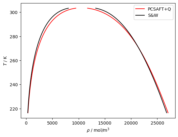
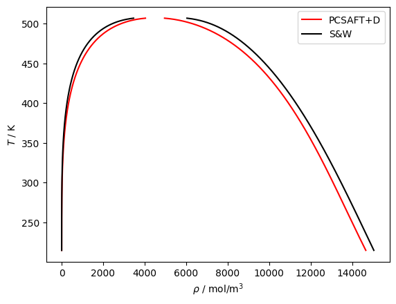
As of teqp version 0.15, quadrupolar and dipolar contributions have been added to the hard chain plus dispersion model which is referred to conventionally as PC-SAFT. The definitions of the reduced dipolar and quadrupolar parameters are not well documented, so they are given here. The work of Stoll, Vrabec, and Hasse (https://doi.org/10.1063/1.1623475) clearly describes the formulation of the star-scaling.

In SI units, the reduced squared dipole moment is defined by

\[(\mu^*)^2_{\rm conventional} = \frac{(\mu[Cm])^2}{4\pi\epsilon_0(\varepsilon[J])(\sigma[m])^3}\]

\[(Q^*)^2_{\rm conventional} = \frac{(Q[Cm^2])^2}{4\pi\epsilon_0(\varepsilon[J])(\sigma[m])^5}\]

In the PC-SAFT formulation, the only difference is the addition of dividing the denominator by the number of segments \(m\)

\[(\mu^*)^2 = \frac{(\mu[Cm])^2}{4\pi\epsilon_0m(\varepsilon/k_{\rm B}[K])k_B(\sigma[m])^3}\]

\[(Q^*)^2 = \frac{(Q[Cm^2])^2}{4\pi\epsilon_0m(\varepsilon/k_B[K])k_B(\sigma[m])^5}\]

The unit conversions are obtained from

\[(\sigma[m]) = (10^{-10}m/A)(\sigma[A])\]

\[(\mu[Cm]) = (3.33564 \times 10^{-30} Cm/D)(\mu[D])\]

and \(\epsilon_0=8.85419e-12\) C\(^2\) N\(^{-1}\) m\(^{-2}\) is the permittivity of vacuum.

[10]:

# CO2 with quadrupolar contributions
j = {
    'kind': 'PCSAFT',
    'model': {
        'coeffs': [{
            'name': 'CO2',
             'BibTeXKey': 'Gross-AICHEJ',
             'm': 1.5131,
             'sigma_Angstrom': 3.1869,
             'epsilon_over_k': 169.33,
             '(Q^*)^2': 1.26, # modified from the values in Gross and Vrabec since the base model is different
             'nQ': 1
        }]
    }
}

model = teqp.make_model(j)
Tc, rhoc = model.solve_pure_critical(300, 11000)

T = Tc*0.999
rhoL_, rhoV_ = model.extrapolate_from_critical(Tc, rhoc, T)
rhoL, rhoV = model.pure_VLE_T(T, rhoL_, rhoV_, 10)

import CoolProp.CoolProp as CP
import matplotlib.pyplot as plt
import pandas
o = []
for T_ in np.linspace(T, 215, 1000):
    rhoL, rhoV = model.pure_VLE_T(T_, rhoL, rhoV, 10)
    try:
        o.append({
          'T': T_, 'rhoL': rhoL, 'rhoV': rhoV,
          'rhoLSW': CP.PropsSI('Dmolar','T',T_,'Q',0,'CO2'),
          'rhoVSW': CP.PropsSI('Dmolar','T',T_,'Q',1,'CO2')
        })
    except:
        pass
df = pandas.DataFrame(o)
plt.plot(df['rhoL'], df['T'], 'r', label='PCSAFT+Q')
plt.plot(df['rhoV'], df['T'], 'r')
plt.plot(df['rhoLSW'], df['T'], 'k', label='S&W')
plt.plot(df['rhoVSW'], df['T'], 'k')
plt.legend()
plt.gca().set(xlabel=r'$\rho$ / mol/m$^3$', ylabel='$T$ / K')
plt.show()

[11]:

# Acetone with dipolar contributions
j = {
    'kind': 'PCSAFT',
    'model': {
        'coeffs': [{
            'name': 'acetone',
             'BibTeXKey': 'Gross-IECR',
             'm': 2.7447,
             'sigma_Angstrom': 3.2742,
             'epsilon_over_k': 232.99,
             '(mu^*)^2': 1.9, # modified from the values in Gross and Vrabec since the base model is different
             'nmu': 1
        }]
    }
}

model = teqp.make_model(j)
Tc, rhoc = model.solve_pure_critical(300, 11000)

T = Tc*0.999
rhoL_, rhoV_ = model.extrapolate_from_critical(Tc, rhoc, T)
rhoL, rhoV = model.pure_VLE_T(T, rhoL_, rhoV_, 10)

import CoolProp.CoolProp as CP
import matplotlib.pyplot as plt
import pandas
o = []
for T_ in np.linspace(T, 215, 1000):
    rhoL, rhoV = model.pure_VLE_T(T_, rhoL, rhoV, 10)
    try:
        o.append({
          'T': T_, 'rhoL': rhoL, 'rhoV': rhoV,
          'rhoLSW': CP.PropsSI('Dmolar','T',T_,'Q',0,'acetone'),
          'rhoVSW': CP.PropsSI('Dmolar','T',T_,'Q',1,'acetone')
        })
    except:
        pass
df = pandas.DataFrame(o)
plt.plot(df['rhoL'], df['T'], 'r', label='PCSAFT+D')
plt.plot(df['rhoV'], df['T'], 'r')
plt.plot(df['rhoLSW'], df['T'], 'k', label='S&W')
plt.plot(df['rhoVSW'], df['T'], 'k')
plt.legend()
plt.gca().set(xlabel=r'$\rho$ / mol/m$^3$', ylabel='$T$ / K')
plt.show()

PC-SAFT¶

Adjusting k_ij¶

Alternative a and b matrices¶

Superancillary¶

Maximum density¶

Polar contributions¶

Table of Contents

Related Topics

This Page