import scipy.interpolate
import teqp
import numpy as np
import pandas
import matplotlib.pyplot as plt
teqp.__version__

'0.22.0'

Critical curves & points

Pure Fluids

Solving for the critical point involves finding the temperature and density that make

\[\left(\frac{\partial p}{\partial \rho}\right)_T = \left(\frac{\partial^2 p}{\partial \rho^2}\right)_T = 0\]

by 2D non-linear rootfinding. Newton steps are taken, and the analytic Jacobian is used (thanks to the ability to do derivatives with automatic differentiation). This is all handily wrapped up in the solve_pure_critical method which requires the user to provide guess values for temperature and density

# Values taken from http://dx.doi.org/10.6028/jres.121.011
modelPR = teqp.canonical_PR([190.564], [4599200], [0.011])

# Solve for the critical point from a point close to the critical point
T0 = 192.0
# Critical compressibility factor of P-R is 0.307401308698.. (see https://doi.org/10.1021/acs.iecr.1c00847)
rhoc = (4599200/(8.31446261815324*190.564))/0.3074
rho0 = rhoc*1.2345 # Perturb to make sure we are doing something in the solver
modelPR.solve_pure_critical(T0, rho0)

(190.564, 9442.816240022832)

If you have a mixture, but want to obtain the critical point of a pure fluid of this mixture, you can specify the index of the component in the mixture, as well as the number of componnts in the mixture with something like:

model.solve_pure_critical(T0, rho0, {"alternative_pure_index": 1, "alternative_length": 2}) so here, for the second fluid, with 0-based index of 1, in a two-component mixture

Mixtures

A pure fluid has a single vapor-liquid critical point, but mixtures are different:

• They may have multiple (or zero!) critical points for a given mixture composition

• The critical curves may not emanate from the pure fluid endpoints

When it comes to critical points, intuition from pure fluids is not helpful, or sometimes even counter-productive.

teqp has methods for working with the critical loci of binary mixtures (only binary mixtures, for now) and especially, methods for tracing the critical curves emanating from the pure fluid endpoints.

The tracing method in teqp is based explicitly on the isochoric thermodynamics formalism introduced by Ulrich Deiters and Sergio Quinones-Cisneros. It uses the Helmholtz energy density as the fundamental potential and all other properties are derived from it. For critical curves it is based upon the integration of sets of ordinary differential equations; the differential equations are in the form of derivatives of the molar concentrations of each component in the mixture with respect to an integration variable. The set of ODE is then integrated.

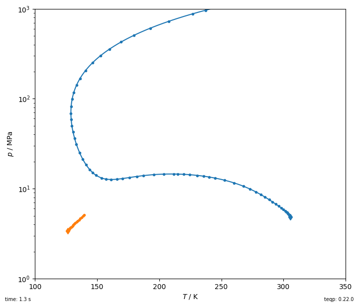
Here is an example of the construction of the critical curves emanating from the pure fluid endpoints for the mixture nitrogen + ethane.

import timeit
import numpy as np
import matplotlib.pyplot as plt
import pandas
import teqp

def get_critical_curve(ipure):
    """ Return curve as pandas DataFrame """
    names = ['Nitrogen', 'Ethane']
    model = teqp.build_multifluid_model(names, teqp.get_datapath())
    T0 = model.get_Tcvec()[ipure]
    rho0 = np.array([1.0/model.get_vcvec()[ipure]]*2)
    rho0[1-ipure] = 0
    o = teqp.TCABOptions()
    o.init_dt = 1.0 # step in the arclength tracing parameter
    o.rel_err = 1e-8
    o.abs_err = 1e-5
    o.integration_order = 5
    o.calc_stability = True
    o.polish = True
    curveJSON = model.trace_critical_arclength_binary(T0, rho0, '', o)
    df = pandas.DataFrame(curveJSON)
    rhotot = df['rho0 / mol/m^3']+df['rho1 / mol/m^3']
    df['z0 / mole frac.'] = df['rho0 / mol/m^3']/rhotot
    return df

fig, ax = plt.subplots(1,1,figsize=(7, 6))
tic = timeit.default_timer()
for ipure in [1,0]:
    df = get_critical_curve(ipure)
    first_unstable = np.argmax(~df['locally stable'])
    df = df.iloc[0:(first_unstable if first_unstable else len(df))]
    line, = plt.plot(df['T / K'], df['p / Pa']/1e6, '.')

    # And interpolate to smooth out the curve using the arclength
    # parameter (which must be monotonically increasing) as
    # the interpolation variable
    tinterp = np.linspace(df['t'].min(), df['t'].max(), 10000)
    Tinterp = scipy.interpolate.interp1d(df['t'], df['T / K'], kind='cubic')(tinterp)
    pinterp = scipy.interpolate.interp1d(df['t'], df['p / Pa'], kind='cubic')(tinterp)
    plt.plot(Tinterp, pinterp/1e6, color=line.get_color())

    plt.plot(df['T / K'].iloc[0], df['p / Pa'].iloc[0]/1e6, 'd',
        color=line.get_color())

elap = timeit.default_timer()-tic
plt.gca().set(xlabel='$T$ / K', ylabel='$p$ / MPa',
    xlim=(100, 350), ylim=(1, 1e3))
plt.yscale('log')
plt.tight_layout(pad=0.2)
plt.gcf().text(0,0,f'time: {elap:0.1f} s', ha='left', va='bottom', fontsize=7)
plt.gcf().text(1,0,f'teqp: {teqp.__version__}', ha='right', va='bottom', fontsize=7);

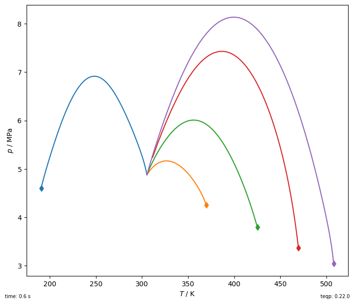
And now for something a bit more interesting: ethane + alkane critical curves

import timeit
import numpy as np
import matplotlib.pyplot as plt
import pandas
import teqp

def get_critical_curve(names, ipure):
    """ Return curve as pandas DataFrame """
    model = teqp.build_multifluid_model(names, teqp.get_datapath())
    T0 = model.get_Tcvec()[ipure]
    rho0 = np.array([1.0/model.get_vcvec()[ipure]]*2)
    rho0[1-ipure] = 0
    o = teqp.TCABOptions()
#     print(dir(o))
    o.init_dt = 1.0 # step in the parameter
    o.rel_err = 1e-6 # relative error on the step
    o.abs_err = 1e-6 # absolute error on the step
    o.max_dt = 100 # cap the size of the allowed step
    o.calc_stability = True
    o.polish = True
    curveJSON = model.trace_critical_arclength_binary(T0, rho0, '', o)
    df = pandas.DataFrame(curveJSON)
    rhotot = df['rho0 / mol/m^3']+df['rho1 / mol/m^3']
    df['z0 / mole frac.'] = df['rho0 / mol/m^3']/rhotot
    return df

fig, ax = plt.subplots(1,1,figsize=(7, 6))
tic = timeit.default_timer()
name0 = 'ETHANE'
for othername in ['METHANE','PROPANE','BUTANE','PENTANE','HEXANE']:
    for ipure in [1]:
        df = get_critical_curve([name0, othername], ipure)
        line, = plt.plot(df['T / K'], df['p / Pa']/1e6, '-')
        plt.plot(df['T / K'].iloc[0], df['p / Pa'].iloc[0]/1e6, 'd',
            color=line.get_color())

elap = timeit.default_timer()-tic
plt.gca().set(xlabel='$T$ / K', ylabel='$p$ / MPa')#,xlim=(100, 350), ylim=(1, 1e3))
plt.tight_layout(pad=0.2)
plt.gcf().text(0,0,f'time: {elap:0.1f} s', ha='left', va='bottom', fontsize=7)
plt.gcf().text(1,0,f'teqp: {teqp.__version__}', ha='right', va='bottom', fontsize=7);

Pure fluid EOS with nonanalytic terms

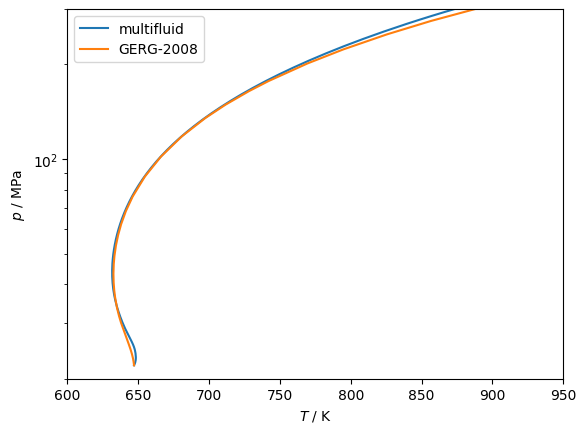
For the highest accuracy EOS for normal water and carbon dioxide, there are non-analytic terms that prevent the initialization of the critical tracing at the pure fluid critical point. Instead, one can start close to, but not AT, the pure fluid endpoint. After deciding on that starting composition, one solves for the critical point and then traces away from it.

You might need to either do tracing in two parts, one with init_c=+1 and then init_c=-1, or one tracing might be good enough.

Here is an example:

def get_critical_curve_composition(names, T0, rhovec0, init_c=-1):
    """ Trace the critical curve from a fixed point along it """
    o = teqp.TCABOptions()
#     print(dir(o))
    o.init_dt = 1.0 # step in the parameter
    o.rel_err = 1e-6 # relative error on the step
    o.abs_err = 1e-6 # absolute error on the step
    o.max_dt = 100 # cap the size of the allowed step
    o.calc_stability = True
    o.polish = True
    o.init_c = init_c # You might need to swap the initial tracing direction by making this +1.0
    curveJSON = model.trace_critical_arclength_binary(T0, rhovec0, '', o)
    df = pandas.DataFrame(curveJSON)
    rhotot = df['rho0 / mol/m^3']+df['rho1 / mol/m^3']
    df['z0 / mole frac.'] = df['rho0 / mol/m^3']/rhotot
    return df

# Tracing with multi-fluid from an endpoint with non-analytic terms
model = teqp.build_multifluid_model(["Water", "Methane"], teqp.get_datapath())

x0 = 1-1e-6 # ever so slightly away from the pure fluid
molefrac = np.array([x0, 1-x0])

# Solve for the actual critical point at this mole fraction with scipy
y0 = [model.get_Tcvec()[0], 1/model.get_vcvec()[0]]
residual = lambda y: model.get_criticality_conditions(y[0], y[1]*molefrac)
res = scipy.optimize.fsolve(residual, y0)
T = res[0]
rho0 = res[1]
rhovec0 = rho0*molefrac

# Now trace from this point
curve = get_critical_curve_composition(model, T0=T, rhovec0=rhovec0)
plt.plot(curve['T / K'], curve['p / Pa']/1e6, label='multifluid')

# With GERG-2008, things are much more straightforward...
model = teqp.make_model({'kind': 'GERG2008resid', 'model': {'names': ['water','methane']}})

def get_critical_curve_simple(model, ipure, T0, rho0):
    """ Trace from a pure fluid... """
    rhovec0 = np.array([0, 0])
    rhovec0[ipure] = rho0
    o = teqp.TCABOptions()
    o.init_dt = 1.0 # step in the arclength tracing parameter
    o.rel_err = 1e-8
    o.abs_err = 1e-5
    o.integration_order = 5
    o.calc_stability = True
    o.polish = True
    curveJSON = model.trace_critical_arclength_binary(T0, rhovec0, '', o)
    df = pandas.DataFrame(curveJSON)
    rhotot = df['rho0 / mol/m^3']+df['rho1 / mol/m^3']
    df['z0 / mole frac.'] = df['rho0 / mol/m^3']/rhotot
    return df

for ifluid in [0]:
    Tci = model.get_Tcvec()[ifluid]
    vci = model.get_vcvec()[ifluid]
    df = get_critical_curve_simple(model, ipure=ifluid, T0=Tci, rho0 = 1.0/vci)
    plt.plot(df['T / K'], df['p / Pa']/1e6, label='GERG-2008')

plt.gca().set(xlabel='$T$ / K', ylabel='$p$ / MPa')
plt.yscale('log')
plt.xlim(600, 950)
plt.ylim(20, 300)
plt.legend(loc='best');

Critical points

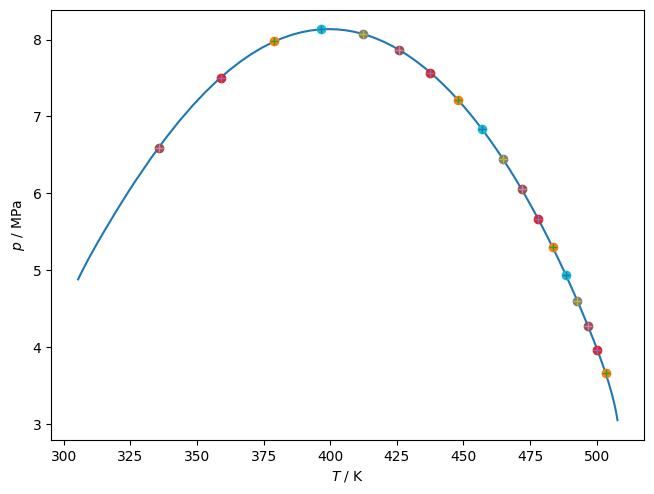
If you have a relatively simple critical curve for a binary mixture and you would like to obtain the critical point at a given composition, you can obtain it reliably in a multi-step process:

1. Trace the binary curve

2. Interpolate to find the approximate value for critical temperature and density

3. Use Newton’s method to solve the criticality conditions from estimated critical point

4. Calculate whatever else you want

df = get_critical_curve([name0, othername], ipure)
model = teqp.build_multifluid_model([name0, othername], teqp.get_datapath())
line, = plt.plot(df['T / K'], df['p / Pa']/1e6, '-')
rhotot = df['rho0 / mol/m^3']+df['rho1 / mol/m^3']

# Build cubic interpolators between the variables
tinterp = scipy.interpolate.interp1d(df['z0 / mole frac.'], df['t'], kind='cubic') # interpolator from mole fraction to tracing parameter
Tinterp = scipy.interpolate.interp1d(df['t'], df['T / K'], kind='cubic')
rhointerp = scipy.interpolate.interp1d(df['t'], rhotot, kind='cubic')

# Iterate over composition
for x0 in np.arange(0.1, 1, 0.05):

    molefracs = np.array([x0, 1-x0])

    # Initial guess for critical point from interpolation
    t = tinterp(x0)
    T0 = Tinterp(t)
    rho0 = rhointerp(t)
    p0 = rho0*model.get_R(molefracs)*T0*(1+model.get_Ar01(T0, rho0, molefracs))
    plt.plot(T0, p0/1e6, 'o')

    # Newton iteration for the correct critical point
    def resid(x):
        return model.get_criticality_conditions(T=x[0], rhovec=x[1]*molefracs)
    soln = scipy.optimize.fsolve(resid, x0=[T0, rho0])
    T, rho = soln
    p = rho*model.get_R(molefracs)*T*(1+model.get_Ar01(T, rho, molefracs))
    plt.plot(T, p/1e6, '+')
#     print(x0, T0, rho0, p0, resid([T0, rho0]), T, rho, resid([T, rho]))

elap = timeit.default_timer()-tic
plt.gca().set(xlabel='$T$ / K', ylabel='$p$ / MPa')
plt.tight_layout(pad=0.2)