Conference Article¶

The following is a conference proceeding published in Reflection, Scattering, and Diffraction from Surfaces VII, SPIE Proc. 11485, 11485-17 (2020). To download this as a Jupyter notebook, click on Show Source and save as “SPIEManuscript.ipynb”, i.e., without “.txt”.

pySCATMECH: A Python interface to the SCATMECH library of scattering codes¶

Thomas A. Germer

Sensor Science Division, National Institute of Standards and Technology, Gaithersburg, Maryland 20899 USA

Abstract: The first version of the SCATMECH polarized light scattering C++ class library was released in 2000. This software provides a large number of models for Mueller matrix bidirectional reflectance distribution function (BRDF), models for free-space scatterers, rigorous coupled wave (RCW) analysis of diffraction gratings, reflectance and transmittance of thin film coatings, and manipulation of polarimetric and optical properties. In 2004, the Modeled Integrated Scatter Tool (MIST) was developed to provide a front-end application for calculating integrated reflectance. While SCATMECH provides efficient codes for modeling, it requires experience with C++ to use, and MIST has limited functionality for many applications. As a result, we have developed a Python interface that provides an intermediate level of access to the SCATMECH library, allowing faster development of applications and test simulations. In this paper, we demonstrate the functionality and use of pySCATMECH using the example of an interference bandpass filter and calculations of scattering by roughness, particles, and volume scattering within that filter.

Keywords: BRDF, interference, modeling, scattering, simulations

1. Introduction¶

Modeling is an important step for interpreting light scattering data. In 2000, after collecting a number of scattering models, we published the SCATMECH C++ library of polarized light scattering codes.[1] SCATMECH is a portmanteau of scattering and mechanics. One of the defining features of the SCATMECH library is that it encapsulated the concept of a model into an abstract class, so that different models for the same quantity can be treated uniformly under a common umbrella. All models have parameters, and in many cases, parameters can be models themselves. For example, a model for rough surface scattering in the smooth surface approximation requires scalar parameters (e.g., wavelength), the optical constants of the material, which are wavelength-dependent, and a power spectral density (PSD) function for the roughness. The PSD is defined by its own model structure, so that a wide variety of PSD functions can be used.

The SCATMECH codes include models for the bidirectional reflectance distribution function (BRDF), for free-space scattering, and for rigourous coupled wave (RCW) analysis of gratings. Each of these models return their respective quantities (e.g., BRDF, differential cross section, or diffraction efficiency, respectively) as Mueller matrices, so that their full polarimetric properties are modeled. Thus, there is an entire module devoted to performing calculations in the Stokes-Mueller formalism, and the library is built around this module.

One drawback to the SCATMECH library is that it is written entirely in C++, making it a significant barrier for many potential users. In fact, while it contains a few simple example programs that can be compiled and executed, the library itself is primarily a class library, requiring additional programming by the user. In 2004, there was interest in being able to calculate the signal expected from spherical reference particles on silicon surfaces collected by specific integrated geometries of wafer surface inspection systems. As a result, we developed the Modeled Integrated Scatter Tool (MIST), [2] which is an executable program. In 2005, MIST was released with a graphical user interface for Microsoft Windows.* MIST thus became the de facto interface to the SCATMECH library. Since it was ultimately designed to perform the integral of the modeled BRDF over an arbitrary collection geometry, in order to estimate the diffuse reflectance, its use in other applications is sometimes awkward. For example, use of RCW models in MIST required that an effective BRDF model be added to SCATMECH, since MIST only works with BRDF models.

There has been a lot of recent attention given to the Python programming language. There are several advantages to Python. First, it is an interpreted language, that can either be run in scripts or executed line by line, making it much easier to develop codes for specific applications, even one-off calculations. Python is freely available, and many extensions are available and easy to install. It has also been incorporated into notebook interfaces, such as Jupyter, allowing for code and visualizations to be interspersed with explanatory text.

As a result, the author has developed a Python interface to the SCATMECH library, called pySCATMECH, for which the first version was be released in July 2020 and can be installed with the common mechanism: pip install pySCATMECH. This manuscript is not intended to fully document pySCATMECH but serves as a set of examples that demonstrate some of its features. The code and documentation are available at [3]. This paper is written and organized as a Jupyter notebook, which will be made available alongside the regular manuscript format.

The organization of this paper is the following: We will construct an interference bandpass filter and show its reflectance properties. We will then consider three mechanisms (models) for light scattering in this film stack. We graph the BRDF at three wavelengths and calculate the diffuse reflectance as a function of wavelength for each of these mechanisms. Finally, we will evalate the integrated cross section of a sphere above the filter as a function of the diameter of the sphere.

*Certain commercial products are identified in this paper in order to specify the procedure adequately. Such identification is not intended to imply recommendation or endorsement by NIST, nor is it intended to imply that these products identified are necessarily the best available for the purpose.

2. First things first¶

Before we start, we need to import the library. Since we will be using some features of the NumPy package and graphing using the PyPlot module of the Matplotlib package, we need to import them as well. Finally, the two symbols pi (for $\pi$) and deg (for $\pi/180$) will be very useful.

In [1]:

from pySCATMECH import fresnel, model, brdf, integrate, local, mueller
import numpy as np
import matplotlib.pyplot as plt
pi = np.pi
deg = pi/180

3. Optical functions¶

We start our examples by creating some optical functions. If we already have tabulated data (i.e., optical constants $n$ and $k$ as functions of wavelength), we can pass the name of the file containing the data as a string to fresnel.OpticalFunction. In this example, we provide Sellmeier expressions for SiO$_2$ (substrate), MgF (low index film), and ZrO$_2$ (high index film) that we will use for our demonstration. [4] [5] [6] Because the underlying SCATMECH code requires optical functions to be provided either as constants or as files, pySCATMECH will create temporary files containing the wavelengths tabulated in some range. Here, we only need to coarsely tabulate the data (20 points over the range 0.35 µm to 0.75 µm) in order to describe the materials.

In [2]:

table_wavelengths = np.linspace(0.350, 0.750, 20)

SiO2 = fresnel.OpticalFunction(
              lambda L: np.sqrt(1 + 0.6961663*L**2/(L**2 - 0.06840432**2)
                                  + 0.4079426*L**2/(L**2 - 0.11624142**2)
                                  + 0.8974794*L**2/(L**2 - 9.8961612**2)),
                                  table_wavelengths)
MgF = fresnel.OpticalFunction(
              lambda L: np.sqrt(1 + 0.48755108*L**2/(L**2 - 0.04338408**2)
                                  + 0.39875031*L**2/(L**2 - 0.09461442**2)
                                  + 2.3120353*L**2/(L**2 - 23.793604**2)),
                                  table_wavelengths)
ZrO2 = fresnel.OpticalFunction(
              lambda L: np.sqrt(1 + 1.347091*L**2/(L**2 - 0.062543**2)
                                  + 2.117788*L**2/(L**2 - 0.166739**2)
                                  + 9.452943*L**2/(L**2 - 24.320570**2)),
                                  table_wavelengths)
vacuum = fresnel.OpticalFunction(1)

4. Interference filter¶

A simple high reflector interference coating consists of alternating high and low index films, each having a quarter-wave thickness at the optimum wavelength. A narrow band interference filter consists of a half-wave thickness layer sandwiched between two high reflectors. For our example, we choose a center wavelength of 0.500 µm and use two five-period high reflectors. We create each film with fresnel.Film. A fresnel.FilmStack, created with a list of fresnel.Film, has a member Rs that returns the reflectance for s-polarization. The example below calculates the reflectance at normal incidence from such a stack on SiO$_2$ as a function of wavelength. The results are shown in Fig. 1. Notice that the device is only a bandpass filter in a narrow range of wavelengths.

In [3]:

L = fresnel.Film(MgF, wavelength = 0.50, waves = 1/4)
H = fresnel.Film(ZrO2, wavelength = 0.50, waves = 1/4)
stack = fresnel.FilmStack(5*[H,L] + [2*L] + 5*[L,H])

wavelengths = np.linspace(0.35, 0.75, 1600)
thetai = 0
reflectance = [stack.Rs(thetai, wavelength, vacuum, SiO2) for wavelength in wavelengths]

plt.figure()
plt.plot(wavelengths,reflectance)
plt.ylabel("Reflectance")
plt.xlabel("Wavelength (µm)")
plt.show()

Figure 1 Reflectance of the interference filter as a function of wavelength.

5. Scattering models¶

We are going to demonstrate scattering from the interference filter described above with three different scattering models, one for random bumps in the interface topography, one for a spherical particle above the stack, and one for small spherical voids randomly placed within the film structure. Figure 2 shows a schematic diagram of the scatterers in the film. Only five films are shown to simplify the figure. In order to compare apples-to-apples, we need to make sure the surface density of the defects and their respective volumes are the same. The volume of a sphere of radius $r$ is $V_\mathrm{sph}=(4/3)\pi r^3$, while that of a parabolic dimple or mound of radius $r$ and height $h$ is $V_\mathrm{int} = \pi r^2 h/2$. For the dimples or mounds, we can specify (as a parameter) their density on each interface, so we should divide the density (here, $\rho$) by the number of interfaces.

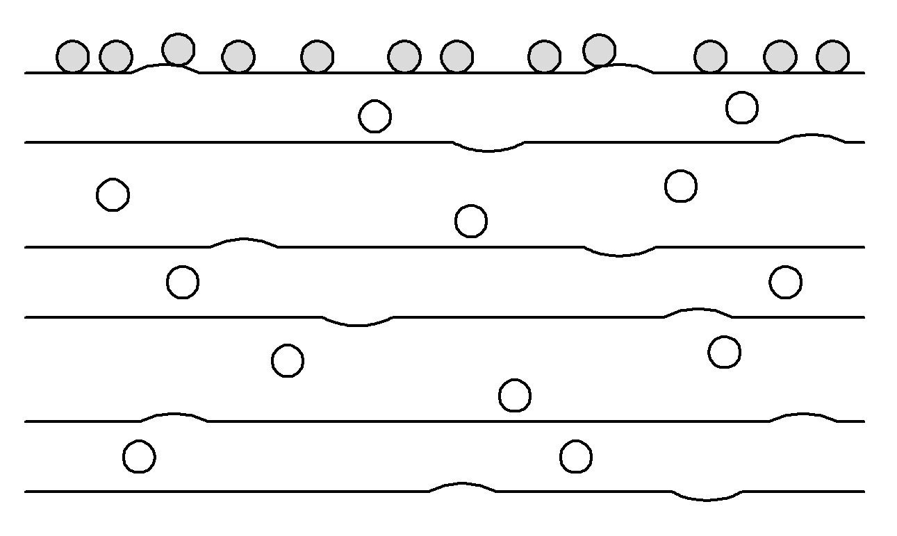
Figure 2: Schematic of the scatterers in the film. Notice that there are the same number of particles on the top, as there are spherical voids distributed within the layers, and dimples or mounds distributed among the interfaces. The number of layers shown is significantly less than that of the filter we are using for the demonstration.

In [4]:

nLayers = len(stack.films)
rho = 1 # in particles per square micrometer

rInterface = 0.25
hInterface = 0.005
rhoInterface = rho / (nLayers+1)
VInterface = pi * rInterface**2 * hInterface/2

rParticle = (3/4 * VInterface / pi)**(1/3)
rhoParticle = rho

rVolume = rParticle
rhoVolume = rho
print("The equivalent particle radius is", rParticle, "µm.")

The equivalent particle radius is 0.048935845514610804 µm.

5.1 Interface roughness¶

We use the model Uncorrelated_Roughness_Stack_BRDF_Model to model the scattering by surface roughness.[7] In this case, we are considering the surfaces to be uncorrelated with one another, but to have identical parabolic dimples or mounds spread between them. In the following, the power spectral density function is defined by psd as a Parabolic_Dimple_PSD_Function.

In [5]:

psd = model.Model('Parabolic_Dimple_PSD_Function',
                  axisx=2*rInterface, axisy=2*rInterface,
                  height=hInterface, density=rhoInterface)
roughnessModel = brdf.BRDF_Model('Uncorrelated_Roughness_Stack_BRDF_Model',
                                 substrate=SiO2, psd=psd, stack=stack)

We should note that it would not be expected that the interfaces be uncorrelated, as shown in Fig. 2. If the surfaces are grown sequentially, a mound or dimple will propagate to some degree to the next interface. Another model Growth_Roughness_Stack_BRDF_Model would be a more realistic model. However, it is more complicated to use and it doesn’t allow for a constant volume comparison between scatterers.

5.2 Particle above the stack¶

We use the theory of Bobbert and Vlieger (BV) to calculate the scatter from spheres above the top interface.[8][9] The BV theory, which is an accurate theory for scattering from a sphere above a substrate, has been extended to include substrates with films.

In [6]:

particleModel = brdf.BRDF_Model('Bobbert_Vlieger_BRDF_Model',
                                substrate=SiO2, density=rhoInterface,
                                sphere=SiO2, radius=rParticle, stack=stack)

5.3 Volume scattering in the stack¶

For scattering from spherical inclusions in a dielectric stack, we use the theory described in Refs. [10] and [11], which is implemented by Rayleigh_Stack_BRDF_Model. The Rayleigh_Stack_BRDF_Model applies to defects at a specific depth in the layer. Therefore, we need to average over the entire depth of the interference stack. Therefore, in the following, we create a new BRDF model, called sumBRDF, which has just the requirements needed for this manuscript, namely an __init__ function to initialize the class, a BRDF function that returns the BRDF, and a setParameters function that allows the parameters to be set once the model has been initialized. In this case, the __init__ function creates the BRDF_Model and determines the total thickness of the stack. The BRDF function averages the BRDF over the depth of the defect, passing the geometry and polarization parameters to the Rayleigh_Stack_BRDF_Model.

In [7]:

class sumBRDF:
    def __init__(self, nstep=20, **parameters):
        self.model = brdf.BRDF_Model('Rayleigh_Stack_BRDF_Model', **parameters)
        self.stack = parameters["stack"]
        self.tthick = sum([f.thickness for f in stack.films])
        self.nstep = nstep

    def BRDF(self, *args, **kwargs):
        zs = np.linspace(0, self.tthick, self.nstep)
        BRDF = 0
        for z in zs:
            self.model.setParameters(depth=z)
            BRDF += self.model.BRDF(*args, **kwargs)
        return BRDF/self.nstep

    def setParameters(self, **kwargs):
        if "nstep" in kwargs:
            self.nstep = kwargs["nstep"]
            del kwargs["nstep"]
        if len(kwargs)>0:
            self.model.setParameters(**kwargs)

volumeModel = sumBRDF(nstep=20, substrate=SiO2, density=rhoVolume,
                      stack=stack, radius=rVolume, sphere=vacuum)

6. BRDF and BTDF¶

Now that we have set up the three models, we can see what the BRDF and bidirectional transmittance distribution function (BTDF) are. As for the SCATMECH library, the BRDF is accessed using the parameter type=0, while BTDF is accessed using type=1. Note that type is a standard function in Python that normally returns the data type of an object. Here type corresponds to the geometry of the measurement. Thus, some care should be taken to not overwrite the standard function. Also, note that the keyword wavelength is used in place of the parameter lambda, which SCATMECH uses for wavelength, since lambda is a dedicated keyword in Python.

In the code below, note that incident polarizations are specified by Stokes vectors or by using specific named polarizations with mueller.Polarization. Similarly, detector sensitivities are specified by Stokes vectors or using named polarizations using mueller.Sensitivity. Using the functions ensures that the result is properly normalized.

The code below calculates the BRDF and BTDF for wavelengths 0.01 µm below, at, and 0.01 µm above the nominal pass wavelength of the filter and for normal incidence, respectively. We use unpolarized incident light with unpolarized sensitivity. In the following block of code, we calculate the bidirectional scattering distribution function (BSDF) for each wavelength and store them in dictionaries.

In [8]:

angles = np.linspace(-89,89,100)

wavelengths = [0.490,0.500,0.510]

inpol = mueller.Polarization('U')
sens = mueller.Sensitivity('U')

roughnessBSDF = dict()
particleBSDF = dict()
volumeBSDF = dict()

for wavelength in wavelengths:
    roughnessBSDF[wavelength] = dict()
    particleBSDF[wavelength] = dict()
    volumeBSDF[wavelength] = dict()
    for BSDFtype in range(2):
        roughnessModel.setParameters(wavelength=wavelength, type=BSDFtype)
        particleModel.setParameters(wavelength=wavelength, type=BSDFtype)
        volumeModel.setParameters(wavelength=wavelength, type=BSDFtype)
        roughnessBSDF[wavelength][BSDFtype] = [
            roughnessModel.BRDF(thetai=0, thetas=t*deg, inc=inpol, sens=sens)
            for t in angles]
        particleBSDF[wavelength][BSDFtype] = [
            particleModel.BRDF(thetai=0, thetas=t*deg, inc=inpol, sens=sens)
            for t in angles]
        volumeBSDF[wavelength][BSDFtype] = [
            volumeModel.BRDF(thetai=0, thetas=t*deg, inc=inpol, sens=sens)
            for t in angles]

The following code does not use any pySCATMECH features, but it graphs the results from the calculations above.

In [9]:

fig, axes = plt.subplots(2,3,figsize=(10,8))

for wavelength in wavelengths:
    for t in range(2):
        axes[t][0].plot(angles, roughnessBSDF[wavelength][t],
                        label="$\lambda=%4.2f$ µm" % wavelength)
        axes[t][1].plot(angles, particleBSDF[wavelength][t],
                        label="$\lambda=%4.2f$ µm" % wavelength)
        axes[t][2].plot(angles, volumeBSDF[wavelength][t],
                        label="$\lambda=%4.2f$ µm" % wavelength)

axes[0][0].set_title("Roughness")
axes[0][1].set_title("Particle")
axes[0][2].set_title("Volume")
axes[0][0].set_ylabel("BRDF (sr$^{-1}$)")
axes[1][0].set_ylabel("BTDF (sr$^{-1}$)")
for row in axes:
    for a in row:
        a.set_yscale('log')
        a.set_xlim((-90, 90))
        a.set_xticks(np.linspace(-90, 90, 5))
for a in axes[1]:
    a.set_xlabel('Angle (°)')
axes[0][0].legend(frameon=False)

plt.show()

Figure 3: The (top row) BRDF and the (bottom row) BTDF calculated for three different models: (left column) roughness of the interfaces, (middle column) spherical particles above the layers, and (right column) spherical voids distributed in the films. The calculations are performed for three wavelengths, 0.49 µm, 0.50 µm, and 0.51 µm.

The BTDFs shown in Fig. 3 are evaluated inside the substrate. Thus, angles outside of approximately 43° are trapped in the substrate.

There are a number of things that can be observed in Fig. 3. Each scattering mechanism is strongly wavelength dependent exhibiting different behavior below, at, and above the nominal wavelength of the filter. For roughness and for volume scattering, the scattering levels are significantly higher at the resonance wavelength. That this is not true for the particles is understandable, since, at the center wavelength, the reflectance of the stack is minimal, and the particle, to some degree does not see the substrate at normal incidence.

The structure observed at 0.49 µm is a result of angle tuning of the filter. At non-normal incidence, the pass wavelength of the filter shifts to shorter wavelength. Thus, there are peaks on each side of the normal viewing direction.

7. Integrated Reflectance¶

In many applications, one is interested in simulating integrated diffuse reflectance. Integration of the BRDF was the primary function of MIST. [2] However, in developing pySCATMECH, we wanted to ensure that this capability was maintained, if not improved. The integrate module of pySCATMECH provides the tools for performing BRDF integration. The first step to using this module is to define the solid angle over which radiation is collected. This is performed by combining a number of different shapes using boolean operations (&, |, and ~). For example, in the following, we define the collection angles by combining the full hemisphere and subtracting (using an “and not” operation) a circular cone (radius of 10°) about the surface normal. The step size at the surface normal is 2° in each direction. The PlotSamplePoints function shows integration points, using symbols sized to indicate the weighting function for integration.

In [10]:

hemisphere = integrate.Hemisphere()
cone = integrate.CircularCone(theta=0*deg, alpha=10*deg)
integrator = integrate.Integrator(2*deg, hemisphere & ~ cone)
integrator.PlotSamplingPoints()

Figure 4: The integration points used in this demonstration, shown as projected cosines, with the surface normal at the center and the plane of incidence being a horizontal line through the center. The area of each point represents the relative weighting factor for each direction.

Once we have the Integrator, we can use it with a BRDF_Model to calculate the reflectance. In the following we calculate the integrated scatter for each of the three scattering mechanisms for an incident angle of 2.5° as a function of wavelength. To assist us, we write a function DiffuseScatter.

In [11]:

def DiffuseScatter(model, wavelengths, type):
    model.setParameters(type=type)
    refs = []
    for wavelength in wavelengths:
        model.setParameters(wavelength=wavelength)
        refs.append(integrator.Reflectance(model, 2.5*deg, incpol=mueller.Polarization('U')))
    return np.array(refs)

wavelengths = np.linspace(0.4, 0.6, 101)

roughnessReflectance = DiffuseScatter(roughnessModel, wavelengths, 0)
particleReflectance = DiffuseScatter(particleModel, wavelengths, 0)
volumeReflectance = DiffuseScatter(volumeModel, wavelengths, 0)
roughnessTransmittance = DiffuseScatter(roughnessModel, wavelengths, 1)
particleTransmittance = DiffuseScatter(particleModel, wavelengths, 1)
volumeTransmittance = DiffuseScatter(volumeModel, wavelengths, 1)

The above code is somewhat time consuming to run, because volumeModel must average over defect depth and there are many directions to sample. In the following, we graph the results.

In [12]:

fig, ((ax1,ax2,ax3),(ax4,ax5,ax6)) = plt.subplots(2,3,figsize=(10,8))

wavelengths = np.linspace(0.4,0.6,101)

ax1.plot(wavelengths,np.array(roughnessReflectance)*1E5)
ax2.plot(wavelengths,np.array(particleReflectance)*1E5)
ax3.plot(wavelengths,np.array(volumeReflectance)*1E5)
ax4.plot(wavelengths,np.array(roughnessTransmittance)*1E5)
ax5.plot(wavelengths,np.array(particleTransmittance)*1E5)
ax6.plot(wavelengths,np.array(volumeTransmittance)*1E5)
ax1.set_ylabel(r"Reflectance $\times 10^5$")
ax4.set_ylabel(r"Transmittance $\times 10^5$")
ax4.set_xlabel("Wavelength (µm)")
ax5.set_xlabel("Wavelength (µm)")
ax6.set_xlabel("Wavelength (µm)")
ax1.set_title("Roughness")
ax2.set_title("Particle")
ax3.set_title("Volume")
plt.show()

Figure 5 The calculated (top row) integrated reflectance and (bottom row) integrated transmittance as a function of wavelength for three different models: (left column) roughness of the interfaces, (middle column) spherical particles above the layers, and (right column) spherical voids distributed in the films. The calculations are performed for an incident angle of 2.5°.

The results are shown in Fig. 5. For the roughness model and the volume scattering model, we can see a strong enhancement in the scattering function at the design wavelength for the filter. For the particle scattering, the effect of the filter bandpass is significantly less. Over the entire spectral range, the scattering is the least for the particles in transmission, which is not too surprising, given that the material is a high reflector at most wavelengths in the region shown.

8. Cross section¶

For isolated defects, the integrated cross section is a more appropriate quantity than BRDF to express the scattering function. In SCATMECH, models inheriting Local_BRDF_Model return the differential cross section for a given geometry, instead of the BRDF. Local_BRDF_Model uses a surface density (as above for particleModel and volumeModel) to determine the BRDF. MIST was able to calculate integrated cross section, but it did so by reverse-engineering that conversion. Thus, it was rather clumsy and confusing to use. In developing pySCATMECH, we make the calculation of the cross section more organic. Those models that inherit Local_BRDF_Model are created as such, so that their differential cross section functions can be accessed.

In the following, we calculate the integrated cross section for scattering by a single sphere on top of the film stack as a function of sphere diameter at the three wavelengths studied above ($:nbsphinx-math:`lambda `= $ 0.49 µm, 0.50 µm, and 0.51 µm). Note that we are spreading the diameters out on a logarithmic scale.

In [13]:

plt.figure()
localParticleModel = local.Local_BRDF_Model('Bobbert_Vlieger_BRDF_Model',
                           wavelength=0.500, substrate=SiO2, type=0, sphere=SiO2, radius=0.05, stack=stack)

wavelengths = [0.490, 0.500, 0.510]
def plotSigmaVsD(model, wavelength):
    model.setParameters(type=0, wavelength=wavelength)

    refs = []
    diameters = np.exp(np.linspace(np.log(0.1), np.log(2), 100))
    for D in diameters:
        model.setParameters(radius=D/2)
        refs.append(integrator.CrossSection(model, 2.5*deg, incpol=mueller.Polarization('U')))
    plt.plot(diameters, refs, label="$\lambda = $%4.2f µm" % wavelength)

for wavelength in wavelengths:
    plotSigmaVsD(localParticleModel, wavelength)

plt.xscale("log")
plt.yscale("log")
plt.xlabel("Diameter (µm)")
plt.ylabel("Cross section (µm$^2$)")
plt.legend(frameon=False)
plt.show()

Figure 6: The cross section for integrated reflective scatter of SiO$_2$ spheres on top of the interference filter as a function of diameter for wavelengths below, at, and above the design wavelength of the filter.

Figure 6 shows the results of the calculations for integrated cross section as a function of sphere diameter $D$. At small diameters, the results show a very strong diameter dependence, significantly greater than $D^6$ (typical for Rayleigh scattering), especially above and below the design wavelength, where the stack is highly reflective. At larger diameters, oscillations in the cross section can be observed. Those oscillations appear stronger above and below the design wavelength. At larger diameter, the curves approach a $D^2$ dependence, due to the geometric cross section being proportional to area.

9. Summary¶

In this proceedings, we introduce pySCATMECH, a Python inteface to the SCATMECH library of scattering models. This manuscript is intended as an introduction and not a full tutorial. Further information can be found in the full documentation [3]. It is anticipated that pySCATMECH will evolve to some degree after its first release. This manuscript is available as a Jupyter notebook located in the documentation. [3]

References

3. pySCATMECH, available online at http://github.com/usnistgov/pySCATMECH.
5. Marilyn J. Dodge, “Refractive properties of magnesium fluoride,” Appl. Opt. 23, 1980-1985 (1984).