K-Marginal Synopsys:
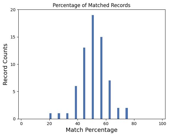
The k-marginal metric checks how far the shape of the deidentified data distribution has shifted away from the target data distribution. It does this using many 3-dimensional snapshots of the data, averaging the density differences across all snapshots. It was developed by Sergey Pogodin as an efficient scoring mechanism for the NIST Temporal Data Challenges, and can be applied to measure the distance between any two data distributions. A score of 0 means two distributions have zero overlap, while a score of 1000 means the two distributions match identically. More information can be found
here.
Sampling Error Comparison:
Here we provide a sampling error baseline: Taking a random subsample of the data also shifts the distribution by introducing sampling error. How does the shift from deidentifying data compare to the shift that would occur from subsampling the target data?
K-Marginal score of the deidentified data closely resembles K-Marginal score of a 30% sub-sample of the target data.
|
Sub-Sample Size
|
Sub-Sample K-Marginal Score
|
Deidentified Data K-marginal score
|
Absolute Diff. From Deidentified Data K-marginal Score
|
| 10% |
844 |
920 |
76 |
| 20% |
894 |
920 |
26 |
| 30% |
913 |
920 |
7 |
| 40% |
929 |
920 |
9 |
| 50% |
943 |
920 |
23 |
| 60% |
951 |
920 |
31 |
| 70% |
957 |
920 |
37 |
| 80% |
968 |
920 |
48 |
| 90% |
979 |
920 |
59 |
| 100% |
1000 |
920 |
80 |
K-Marginal Score in Each PUMA:
Different PUMA have different subpopulations and distributions; how much has each PUMA shifted during deidentification?
Univariate Distributions:
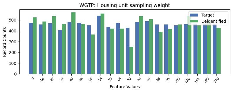
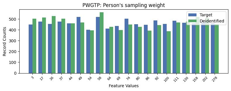
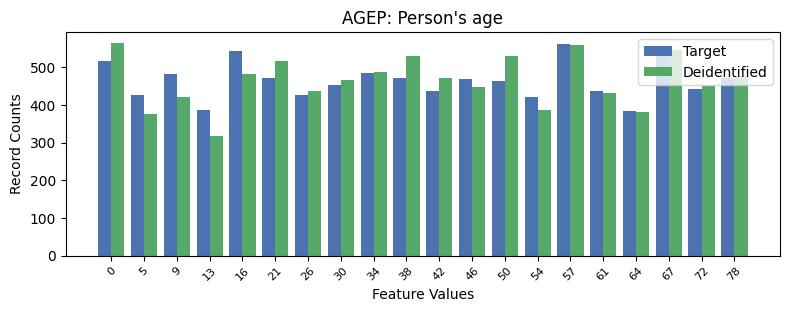
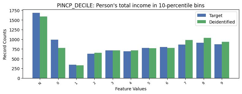
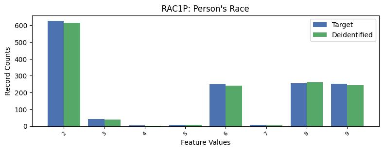
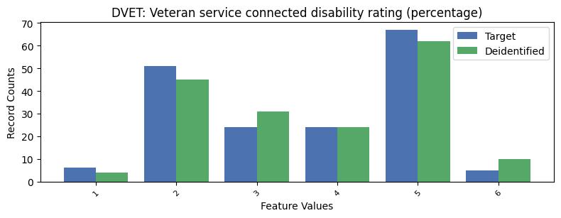
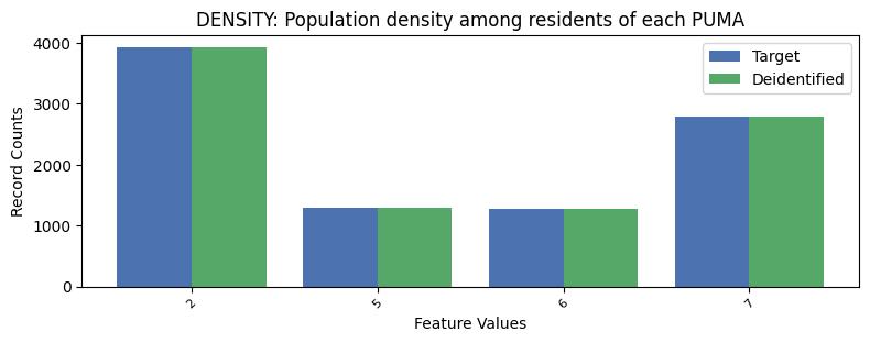
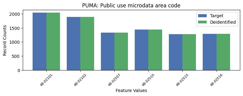
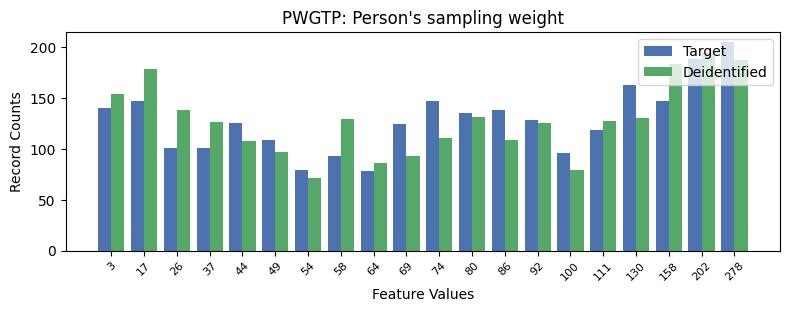
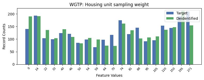
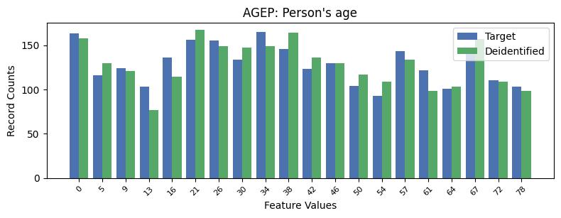
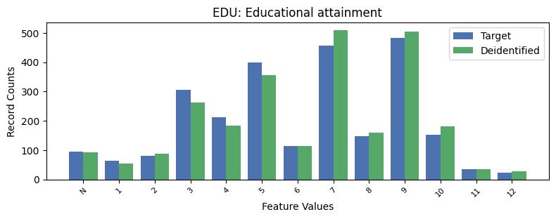
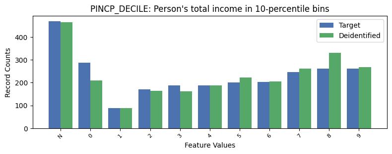
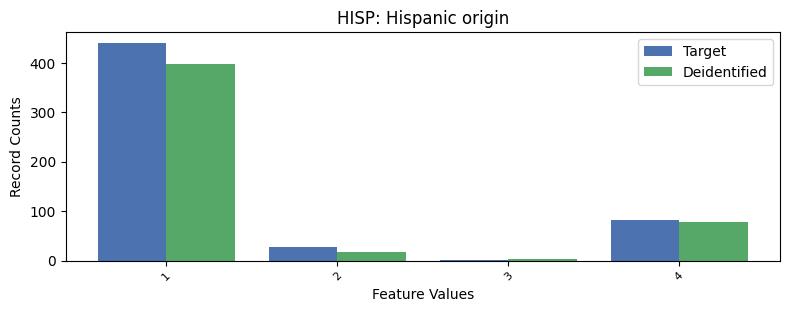
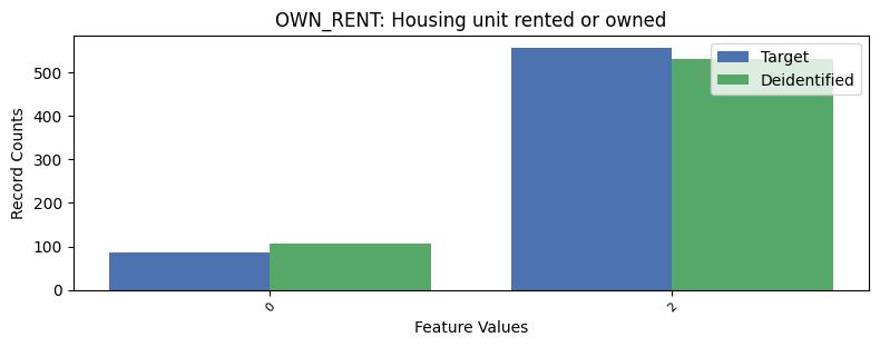
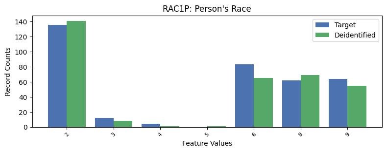
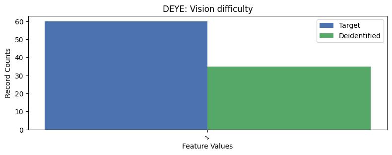
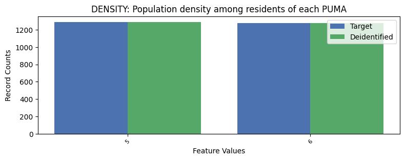
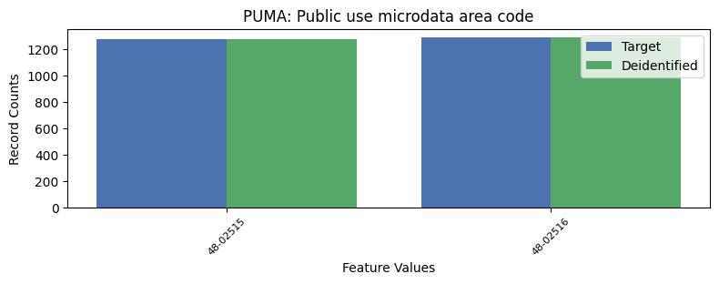
Here we provide single feature distribution comparisons ordered to show worst performing features first (based on the L1 norm of density differences).
WGTP: Housing unit sampling weight:
PWGTP: Person's sampling weight:
PINCP_DECILE: Person's total income in 10-percentile bins:
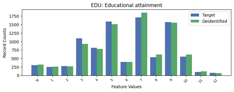
EDU: Educational attainment:
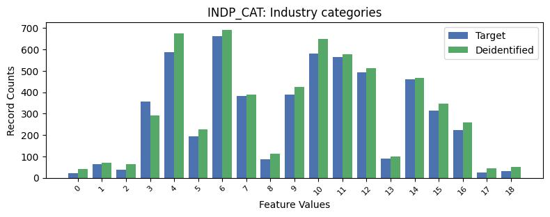
INDP_CAT: Industry categories:
Feature Value: N (N/A)
Target Data Counts: 3714
Deidentified Data Counts: 3289
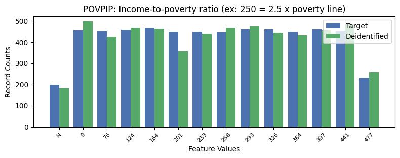
POVPIP: Income-to-poverty ratio (ex: 250 = 2.5 x poverty line):
Feature Value: 501 (Not in poverty: income above 5 x poverty line)
Target Data Counts: 3401
Deidentified Data Counts: 3448
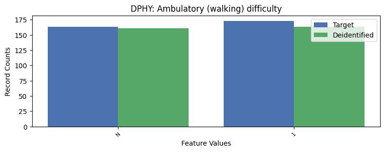
DPHY: Ambulatory (walking) difficulty:
Feature Value: 2
Target Data Counts: 8117
Deidentified Data Counts: 8139
OWN_RENT: Housing unit rented or owned:
Feature Value: 1
Target Data Counts: 7243
Deidentified Data Counts: 7159
Feature Value: 0
Target Data Counts: 7581
Deidentified Data Counts: 7653
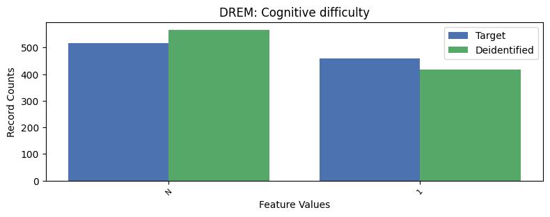
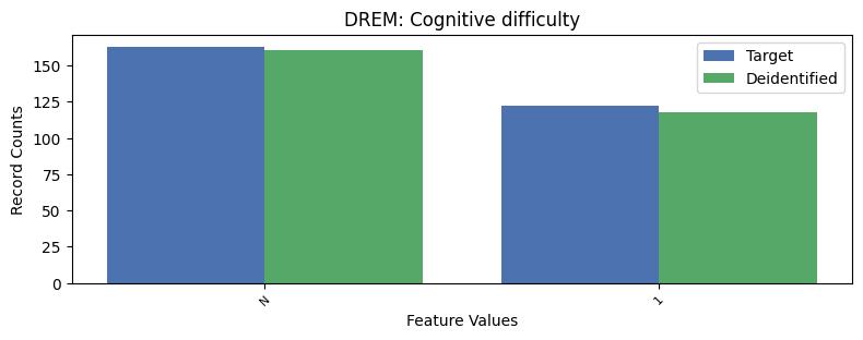
DREM: Cognitive difficulty:
Feature Value: 2
Target Data Counts: 8300
Deidentified Data Counts: 8291
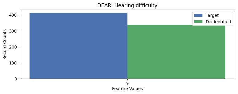
DEAR: Hearing difficulty:
Feature Value: 2
Target Data Counts: 8865
Deidentified Data Counts: 8938
Feature Value: 2
Target Data Counts: 9054
Deidentified Data Counts: 9126
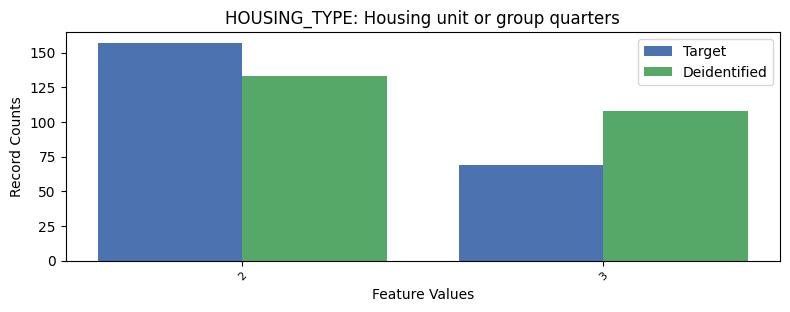
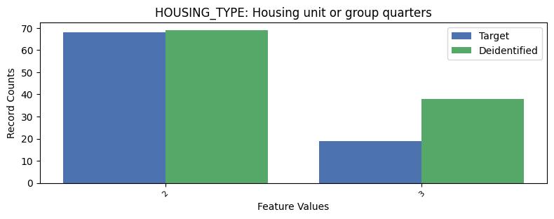
HOUSING_TYPE: Housing unit or group quarters:
Feature Value: 1
Target Data Counts: 9050
Deidentified Data Counts: 9035
Feature Value: 1
Target Data Counts: 7831
Deidentified Data Counts: 7861
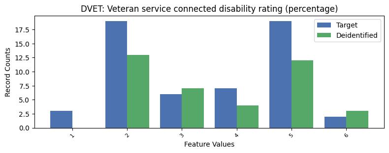
DVET: Veteran service connected disability rating (percentage):
Feature Value: N (N/A)
Target Data Counts: 9099
Deidentified Data Counts: 9100
DENSITY: Population density among residents of each PUMA:
PUMA: Public use microdata area code:
Linear Regression:
Linear regression is a fundamental data analysis technique that condenses a multi-dimensional data distribution down to a one dimensional (line) representation. It works by finding the line that sits in the 'middle' of the data, in some sense--
it minimizes the total distance between the points of the data and the line. There are more advanced forms of regression, but here we're focusing on the simplest case-- we fit a simple straight line to the data, getting the slope and y-intercept value of that line.
For this metric we're just looking at data from adults (AGEP > 15) and we're only considering the distribution of the data across two features:
- EDU: The highest education level this individual has attained, ranging from 1 (elementary school) to 12 (PhD). See Appendix of this report for the full list of code values.
- PINCP_DECILE: The individual's income decile relative to their PUMA. This helps us account for differences in cost of living across the country. If an individual makes a moderate income but lives in a very low income area, they may have a high value for PINCP_DECILE indicating that they have a high income for their PUMA).
The basic idea is that higher values of EDU should lead to higher values of PINCP_DECILE, and this is broadly true. However, it is known that the relationship between EDU and PINCP_DECILE is different for different demographic subgroups. The heatmaps in the left column below show the density distribution of the true data for each subgroup, normalized by education category (so the density values in each column sum to 1; note that when a cell in the heatmap contains too few people (< 20 ), it is left blank; its not expected that the deidentified data will match the original distribution precisely). The regression line is drawn in red over the heatmap, so you can see the relationship between the target data distribution and its linear regression analysis. In the right column for each subgroup we show how the deidentified data's regression line compares to the target data's regression line, along with a heatmap of the density differences between the two distributions. Redder areas are where the deidentified data has created too many people, bluer areas are where it's created too few people.
We've broken this metric down into demographic subgroups so we can see not only how well the privacy techniques preserve the overall relationship between these features, but also whether they preserve how that overall relationship is built up from the different relationships that hold at each major demographic subgroup. It's important that deidentification techniques preserve these distinct subgroup patterns for analysis.
Total Population:
Target Data:
7594 records, 100.0% of adult (>15) data
Regression: 0.58 slope, 0.79 intercept
Deidentified Data:
7686 records, 100.0% of adult (>15) data
Regression: 0.53 slope, 1.37 intercept
White Men:
Target Data:
3128 records, 41.19% of adult (>15) data
Regression: 0.62 slope, 1.48 intercept
Deidentified Data:
3146 records, 40.93% of adult (>15) data
Regression: 0.55 slope, 1.97 intercept
White Women:
Target Data:
3351 records, 44.13% of adult (>15) data
Regression: 0.57 slope, 0.19 intercept
Deidentified Data:
3453 records, 44.93% of adult (>15) data
Regression: 0.53 slope, 0.81 intercept
Black Men:
Target Data:
236 records, 3.11% of adult (>15) data
Regression: 0.79 slope, -0.96 intercept
Deidentified Data:
213 records, 2.77% of adult (>15) data
Regression: 0.6 slope, 0.87 intercept
Black Women:
Target Data:
265 records, 3.49% of adult (>15) data
Regression: 0.68 slope, -0.6 intercept
Deidentified Data:
290 records, 3.77% of adult (>15) data
Regression: 0.58 slope, -0.03 intercept
Asian Men:
Target Data:
94 records, 1.24% of adult (>15) data
Regression: 0.63 slope, 0.06 intercept
Deidentified Data:
104 records, 1.35% of adult (>15) data
Regression: 0.51 slope, 1.61 intercept
Asian Women:
Target Data:
119 records, 1.57% of adult (>15) data
Regression: 0.33 slope, 1.51 intercept
Deidentified Data:
102 records, 1.33% of adult (>15) data
Regression: 0.65 slope, -0.63 intercept
American Indian, Alaskan Native and Native Hawaiians (AIANNH) Men:
Target Data:
19 records, 0.25% of adult (>15) data
Regression: 0.64 slope, 0.42 intercept
Deidentified Data:
17 records, 0.22% of adult (>15) data
Regression: 0.42 slope, 2.95 intercept
American Indian, Alaskan Native and Native Hawaiians (AIANNH) Women:
Target Data:
31 records, 0.41% of adult (>15) data
Regression: 0.61 slope, -0.46 intercept
Deidentified Data:
24 records, 0.31% of adult (>15) data
Regression: 0.84 slope, -1.52 intercept
PCA:
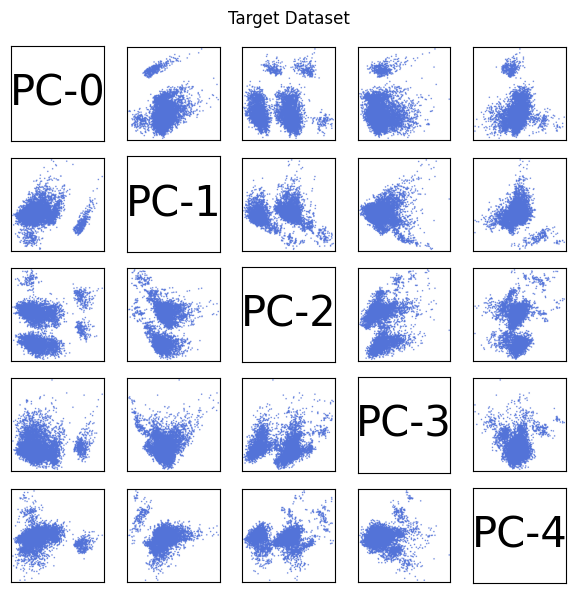
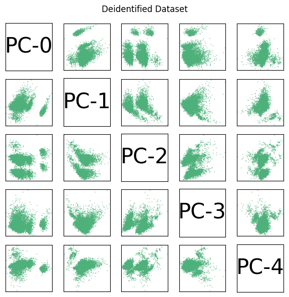
This is another approach for visualizing where the distribution of the deidentified data has shifted away from the target data. In this approach, we begin by using
Principle Component Analysis to find a way of representing the target data in a lower dimensional space (in 5 dimensions rather than the full 22 dimensions of the original feature space). Descriptions of these new five dimensions (components) are given in the components table; the components will change depending on which target data set you�re using. Five dimensions are better than 22, but we actually want to get down to two dimensions so we can plot the data on simple (x,y) axes� the plots below show the data across each possible pair combination of our five components. You can compare how the shapes change between the target data and the deidentified data, and consider what that might mean in light of the component definitions. This is a relatively new visualization metric that was introduced by the
IPUMS International team during the HLG-MOS Synthetic Data Test Drive.
Contribution of Features in Each Principal Component:
|
Principal Component
|
Features Contribution: feature-name (contribution ratio)
|
| PC-0 |
PWGTP (0.15),WGTP (0.15),HISP (0.11),OWN_RENT (0.1),RAC1P (0.08) |
| PC-1 |
WGTP (0.52),PWGTP (0.5),OWN_RENT (0.33),DPHY (0.21),DREM (0.2) |
| PC-2 |
DENSITY (0.64),PUMA (0.64),POVPIP (0.24),HOUSING_TYPE (0.18),RAC1P (0.08) |
| PC-3 |
PWGTP (0.44),WGTP (0.41),HOUSING_TYPE (0.33),POVPIP (0.22),AGEP (0.17) |
| PC-4 |
HOUSING_TYPE (0.4),DEAR (0.36),DEYE (0.26),POVPIP (0.26),DPHY (0.24) |
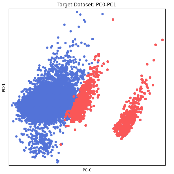
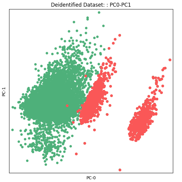
The queries below explore the PCA metric results in more detail by zooming in on a single component-pair panel and highlighting all individuals that satisfy a given constraint (such as MSP = �N�, individuals who are unmarried because they are children). If the deidentified data preserves the structure and feature correlations of the target data, the highlighted areas should have similar shape.
MSP_N: Children (AGEP < 15):
Inconsistencies:
Summary:
|
Inconsistency Group
|
Number of Records Inconsistent
|
Percent Records Inconsistent
|
| Age |
15 |
0.2% |
| Work |
0 |
0.0% |
| Housing |
1 |
0.0% |
Age-Based Inconsistencies:
These inconsistencies deal with the AGE feature; records with age-based inconsistencies might have children who are married, or infants with high school diplomas
child_MSP: Children (< 15) can't be married:
|
AGEP
|
DEAR
|
DENSITY
|
DEYE
|
DPHY
|
DREM
|
DVET
|
EDU
|
HISP
|
HOUSING_TYPE
|
INDP_CAT
|
MSP
|
OWN_RENT
|
PINCP_DECILE
|
POVPIP
|
PUMA
|
PWGTP
|
RAC1P
|
SEX
|
WGTP
|
| 13 |
2 |
7 |
2 |
2 |
2 |
N |
4 |
0 |
1 |
N |
6 |
1 |
0 |
224 |
48-02507 |
63 |
6 |
1 |
86 |
child_PINCP_DECILE: Children (< 15) don't have personal incomes:
|
AGEP
|
DEAR
|
DENSITY
|
DEYE
|
DPHY
|
DREM
|
DVET
|
EDU
|
HISP
|
HOUSING_TYPE
|
INDP_CAT
|
MSP
|
OWN_RENT
|
PINCP_DECILE
|
POVPIP
|
PUMA
|
PWGTP
|
RAC1P
|
SEX
|
WGTP
|
| 13 |
2 |
7 |
2 |
2 |
2 |
N |
4 |
0 |
1 |
N |
6 |
1 |
0 |
224 |
48-02507 |
63 |
6 |
1 |
86 |
child_INDP_CAT: Children (< 15) don't have work industries:
|
AGEP
|
DEAR
|
DENSITY
|
DEYE
|
DPHY
|
DREM
|
DVET
|
EDU
|
HISP
|
HOUSING_TYPE
|
INDP_CAT
|
MSP
|
OWN_RENT
|
PINCP_DECILE
|
POVPIP
|
PUMA
|
PWGTP
|
RAC1P
|
SEX
|
WGTP
|
| 14 |
2 |
5 |
2 |
2 |
2 |
N |
4 |
1 |
1 |
14 |
N |
1 |
N |
272 |
48-02516 |
277 |
1 |
1 |
259 |
adult_N: Adults ( > 14) must specify values (other than N) for all adult features:
|
AGEP
|
DEAR
|
DENSITY
|
DEYE
|
DPHY
|
DREM
|
DVET
|
EDU
|
HISP
|
HOUSING_TYPE
|
INDP_CAT
|
MSP
|
OWN_RENT
|
PINCP_DECILE
|
POVPIP
|
PUMA
|
PWGTP
|
RAC1P
|
SEX
|
WGTP
|
| 17 |
2 |
7 |
2 |
2 |
2 |
N |
3 |
4 |
1 |
N |
N |
1 |
N |
305 |
48-02510 |
165 |
1 |
1 |
103 |
toddler_DPHY: Toddlers (< 5) naturally toddle, it's not a physical disability:
|
AGEP
|
DEAR
|
DENSITY
|
DEYE
|
DPHY
|
DREM
|
DVET
|
EDU
|
HISP
|
HOUSING_TYPE
|
INDP_CAT
|
MSP
|
OWN_RENT
|
PINCP_DECILE
|
POVPIP
|
PUMA
|
PWGTP
|
RAC1P
|
SEX
|
WGTP
|
| 4 |
2 |
2 |
2 |
2 |
2 |
N |
1 |
0 |
1 |
N |
N |
1 |
N |
174 |
48-02101 |
131 |
9 |
1 |
92 |
toddler_DREM: Toddlers (< 5) are naturally forgetful, it's not a cognitive disability:
|
AGEP
|
DEAR
|
DENSITY
|
DEYE
|
DPHY
|
DREM
|
DVET
|
EDU
|
HISP
|
HOUSING_TYPE
|
INDP_CAT
|
MSP
|
OWN_RENT
|
PINCP_DECILE
|
POVPIP
|
PUMA
|
PWGTP
|
RAC1P
|
SEX
|
WGTP
|
| 4 |
2 |
2 |
2 |
2 |
2 |
N |
1 |
0 |
1 |
N |
N |
1 |
N |
174 |
48-02101 |
131 |
9 |
1 |
92 |
Work-Based Inconsistencies:
These inconsistencies deal with the work and finance features; records with work-based inconsistencies might have high incomes while being in poverty, or have conflicts between their industry code and industry category.
Housing-Based Inconsistencies:
These inconsistencies deal with housing and family features; records with household-based inconsistencies might have more children in the house than the total household size, or be residents of group quarters (such as prison inmates) who are listed as owning their residences.
house_OWN_RENT: Individuals who live in houses must specify if they rent or own:
|
AGEP
|
DEAR
|
DENSITY
|
DEYE
|
DPHY
|
DREM
|
DVET
|
EDU
|
HISP
|
HOUSING_TYPE
|
INDP_CAT
|
MSP
|
OWN_RENT
|
PINCP_DECILE
|
POVPIP
|
PUMA
|
PWGTP
|
RAC1P
|
SEX
|
WGTP
|
| 20 |
2 |
2 |
2 |
2 |
2 |
N |
7 |
1 |
1 |
12 |
2 |
0 |
2 |
53 |
48-02101 |
194 |
9 |
2 |
90 |
K-Marginal Score Breakdown:
In the metrics above we�ve considered all of the data together; however we know that algorithms may behave differently on different subgroups in the population. Below we look in more detail at deidentification performance just in the worst performing PUMA, based on k-marginal score.
2 Worst Performing PUMA:
Which are the worst performing PUMA?
Record Counts in 2 Worst Performing PUMA:
Did the deidentified versions of these PUMA have similar population totals to the target versions?
|
Dataset
|
Record Counts
|
| Target |
2567 |
| Deidentified |
2567 |
Univariate Distribution of Worst Performing Features in 2 Worst Performing PUMA:
Which features are performing the worst in each of these PUMA?
PWGTP: Person's sampling weight:
WGTP: Housing unit sampling weight:
EDU: Educational attainment:
PINCP_DECILE: Person's total income in 10-percentile bins:
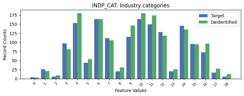
INDP_CAT: Industry categories:
Feature Value: N (N/A)
Target Data Counts: 1031
Deidentified Data Counts: 910
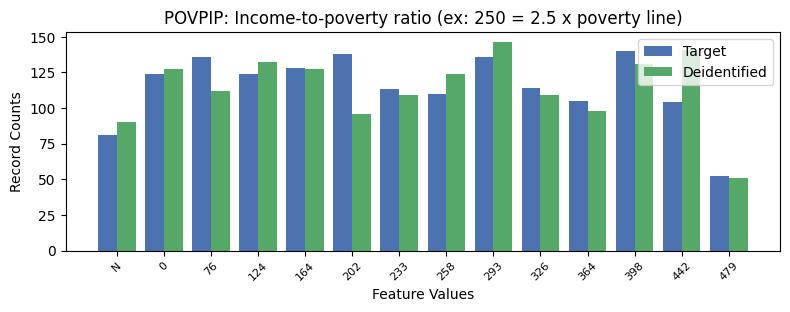
POVPIP: Income-to-poverty ratio (ex: 250 = 2.5 x poverty line):
Feature Value: 501 (Not in poverty: income above 5 x poverty line)
Target Data Counts: 962
Deidentified Data Counts: 974
Feature Value: 0
Target Data Counts: 2016
Deidentified Data Counts: 2071
OWN_RENT: Housing unit rented or owned:
Feature Value: 1
Target Data Counts: 1923
Deidentified Data Counts: 1930
Feature Value: 1
Target Data Counts: 2206
Deidentified Data Counts: 2227
Feature Value: 2
Target Data Counts: 2507
Deidentified Data Counts: 2532
HOUSING_TYPE: Housing unit or group quarters:
Feature Value: 1
Target Data Counts: 2480
Deidentified Data Counts: 2460
DVET: Veteran service connected disability rating (percentage):
Feature Value: N (N/A)
Target Data Counts: 2511
Deidentified Data Counts: 2528
DEAR: Hearing difficulty:
Feature Value: 2
Target Data Counts: 2465
Deidentified Data Counts: 2482
DPHY: Ambulatory (walking) difficulty:
Feature Value: 2
Target Data Counts: 2231
Deidentified Data Counts: 2243
DREM: Cognitive difficulty:
Feature Value: 2
Target Data Counts: 2282
Deidentified Data Counts: 2288
DENSITY: Population density among residents of each PUMA:
PUMA: Public use microdata area code:
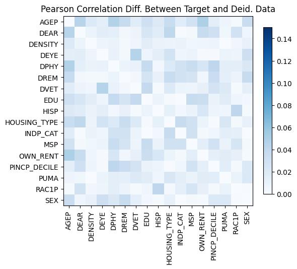
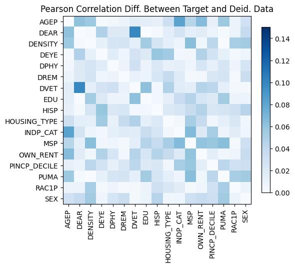
Pearson Correlation Coefficient Difference in 2 Worst Performing PUMA:
How are feature correlations performing in each of these PUMA?
