Data Evaluation Report

Data Evaluation Report


Report created on: March 15, 2023 21:47:56

Created with SDNIST v2.1.0

Data Description

Deidentified (Deid.) Data:

Label Name Label Value
Team MOSTLY AI
Submission Timestamp 3/10/2023 8:29:44
Algorithm Name MOSTLY AI SD Platform
Variant Label national2019_synthetic_s1


Property Value
Filename MostlyAI_sd_platform_PaulTiwald
Records 27253
Features 21

Following features has out of bound values, and these are not used in the evaluations.

Dropped Feature Out of Bound Values
PINCP '_RARE_'
INDP '_RARE_'
NOC 11

Target Data:


Property Value
Filename national2019
Records 27253
Features 24

Evaluated Data Features:

Feature Name Feature Description Feature Type Feature Has 'N' (N/A) values?
PUMA Public use microdata area code object of type string False
AGEP Person's age int64 False
SEX Person's gender int64 False
MSP Marital Status object of type string True
HISP Hispanic origin int64 False
RAC1P Person's Race int64 False
NPF Number of persons in family (unweighted) object of type string True
HOUSING_TYPE Housing unit or group quarters int64 False
OWN_RENT Housing unit rented or owned int64 False
DENSITY Population density among residents of each PUMA float64 False
INDP_CAT Industry categories object of type string True
EDU Educational attainment object of type string True
PINCP_DECILE Person's total income in 10-percentile bins object of type string True
POVPIP Income-to-poverty ratio (ex: 250 = 2.5 x poverty line) object of type string True
DVET Veteran service connected disability rating (percentage) object of type string True
DREM Cognitive difficulty object of type string True
DPHY Ambulatory (walking) difficulty object of type string True
DEYE Vision difficulty int32 False
DEAR Hearing difficulty int32 False
WGTP Housing unit sampling weight int64 False
PWGTP Person's sampling weight int64 False

Utility Evaluation

K-Marginal Synopsys:


The k-marginal metric checks how far the shape of the deidentified data distribution has shifted away from the target data distribution. It does this using many 3-dimensional snapshots of the data, averaging the density differences across all snapshots. It was developed by Sergey Pogodin as an efficient scoring mechanism for the NIST Temporal Data Challenges, and can be applied to measure the distance between any two data distributions. A score of 0 means two distributions have zero overlap, while a score of 1000 means the two distributions match identically. More information can be found here.

K-Marginal Score: 916

Sampling Error Comparison:

Here we provide a sampling error baseline: Taking a random subsample of the data also shifts the distribution by introducing sampling error. How does the shift from deidentifying data compare to the shift that would occur from subsampling the target data?

K-Marginal score of the deidentified data closely resembles K-Marginal score of a 30% sub-sample of the target data.

Sub-Sample Size Sub-Sample K-Marginal Score Deidentified Data K-marginal score Absolute Diff. From Deidentified Data K-marginal Score
10% 839 916 77
20% 891 916 25
30% 913 916 3
40% 926 916 10
50% 937 916 21
60% 947 916 31
70% 957 916 41
80% 967 916 51
90% 977 916 61
100% 1000 916 84

K-Marginal Score in Each PUMA:

Different PUMA have different subpopulations and distributions; how much has each PUMA shifted during deidentification?


Univariate Distributions:


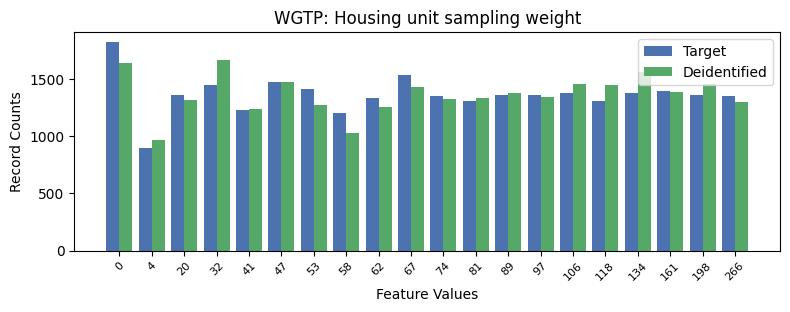
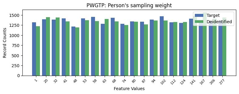
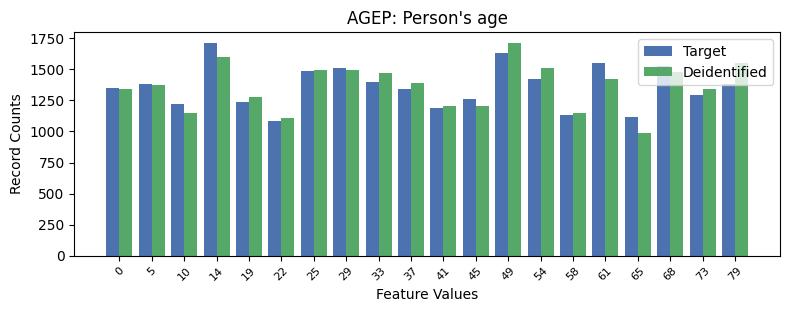
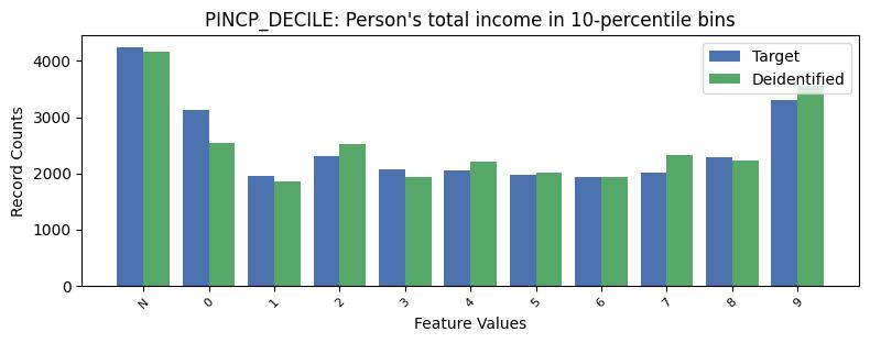
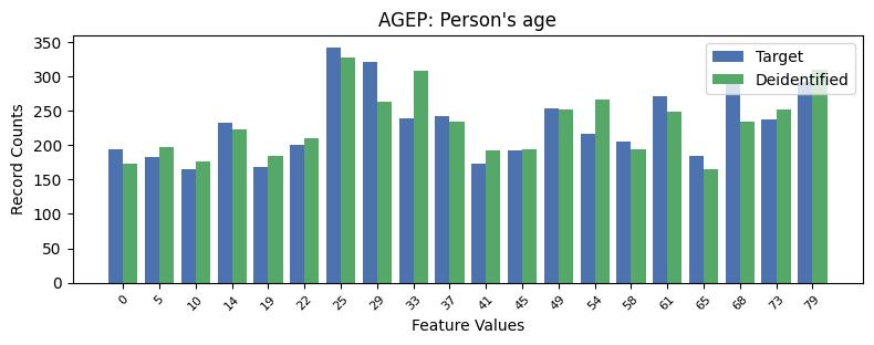
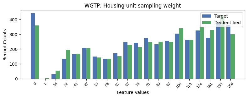
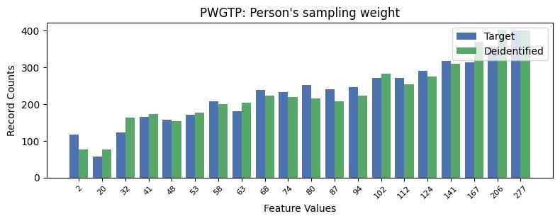
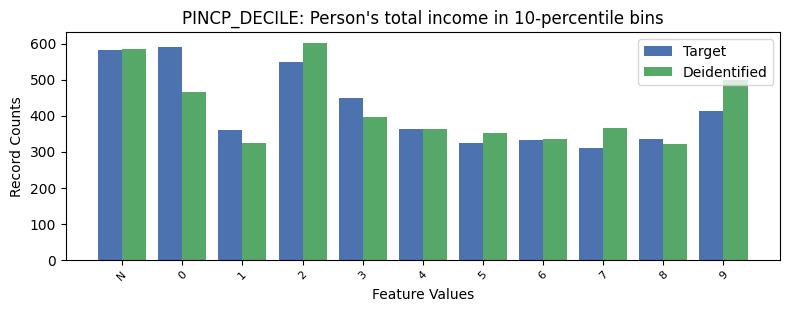
Here we provide single feature distribution comparisons ordered to show worst performing features first (based on the L1 norm of density differences).

WGTP: Housing unit sampling weight:


WGTP

PWGTP: Person's sampling weight:


PWGTP

AGEP: Person's age:


AGEP

PINCP_DECILE: Person's total income in 10-percentile bins:


PINCP_DECILE

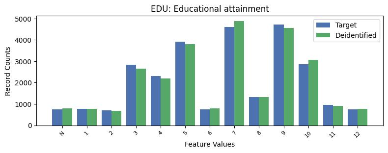
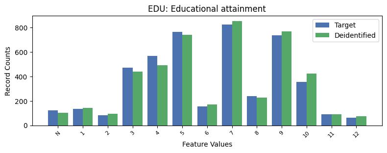
EDU: Educational attainment:


EDU

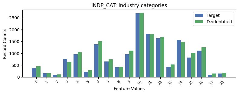
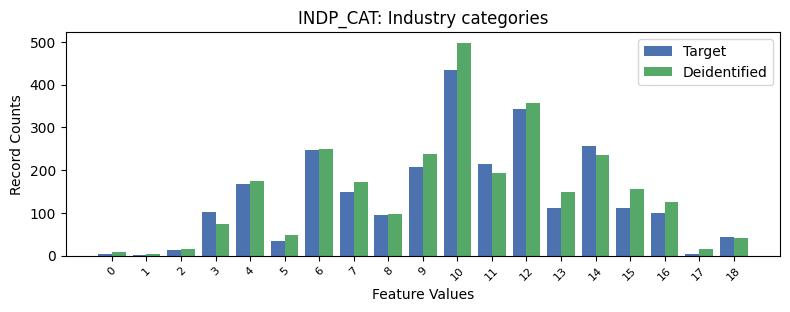
INDP_CAT: Industry categories:


Feature Value: N (N/A)
Target Data Counts: 10929
Deidentified Data Counts: 9965

INDP_CAT

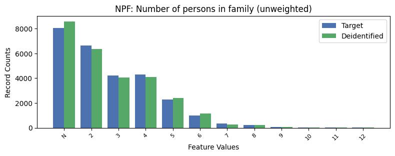
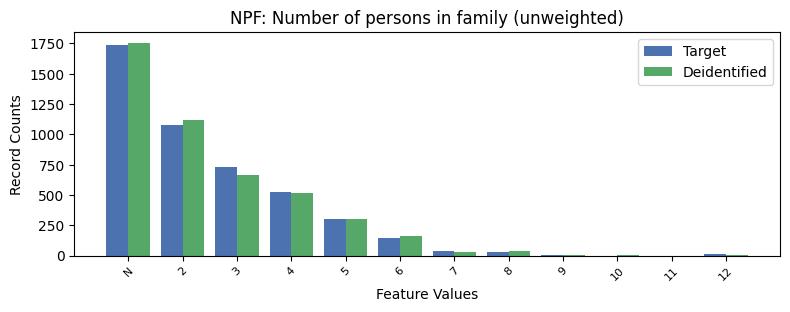
NPF: Number of persons in family (unweighted):


NPF

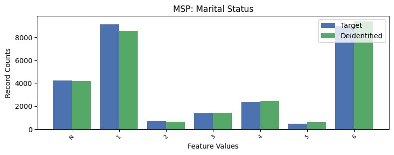
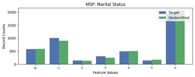
MSP: Marital Status:


MSP

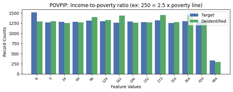
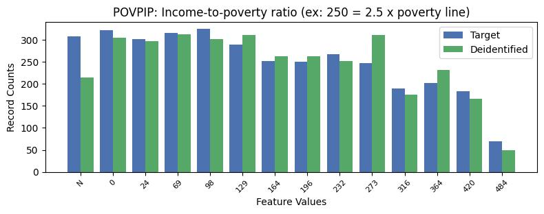
POVPIP: Income-to-poverty ratio (ex: 250 = 2.5 x poverty line):


Feature Value: 501 (Not in poverty: income above 5 x poverty line)
Target Data Counts: 9972
Deidentified Data Counts: 9682

POVPIP

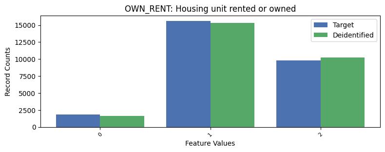
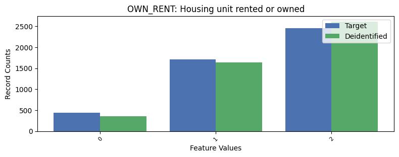
OWN_RENT: Housing unit rented or owned:


OWN_RENT

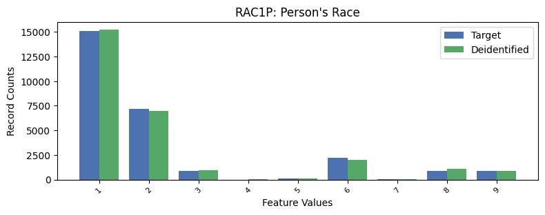
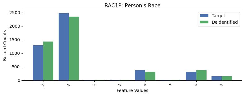
RAC1P: Person's Race:


RAC1P

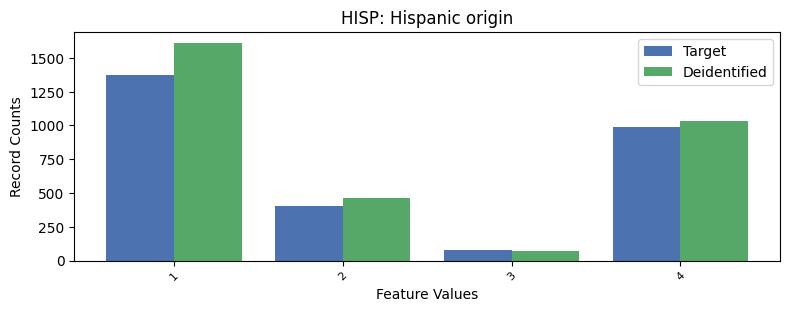
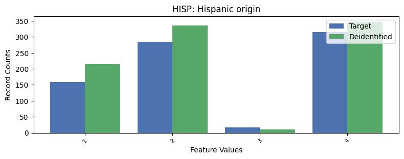
HISP: Hispanic origin:


Feature Value: 0
Target Data Counts: 24400
Deidentified Data Counts: 24079

HISP

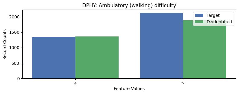
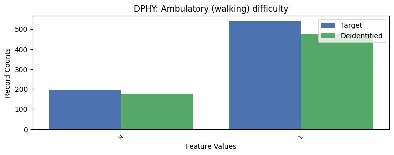
DPHY: Ambulatory (walking) difficulty:


Feature Value: 2
Target Data Counts: 23776
Deidentified Data Counts: 24008

DPHY

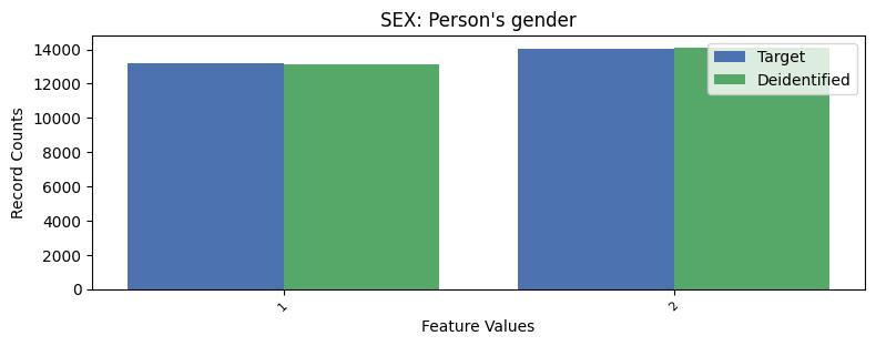
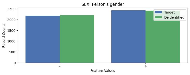
SEX: Person's gender:


SEX

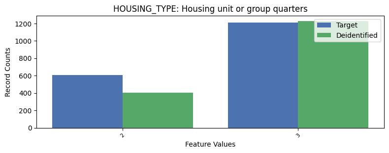
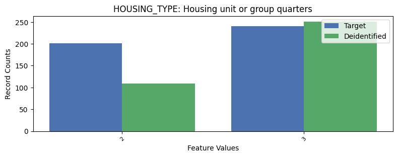
HOUSING_TYPE: Housing unit or group quarters:


Feature Value: 1
Target Data Counts: 25435
Deidentified Data Counts: 25621

HOUSING_TYPE

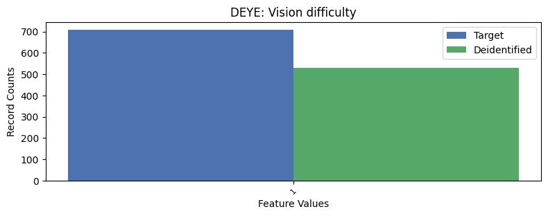
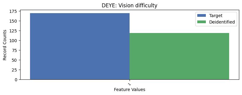
DEYE: Vision difficulty:


Feature Value: 2
Target Data Counts: 26544
Deidentified Data Counts: 26723

DEYE

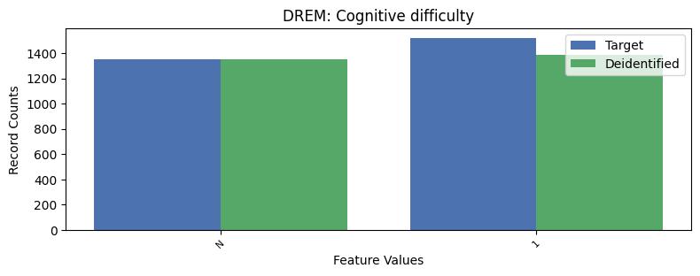
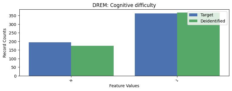
DREM: Cognitive difficulty:


Feature Value: 2
Target Data Counts: 24379
Deidentified Data Counts: 24517

DREM

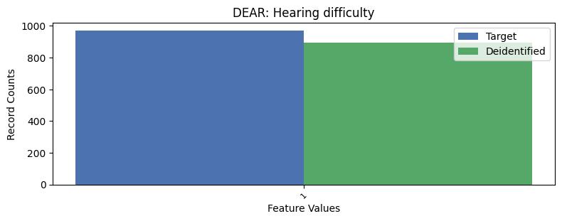
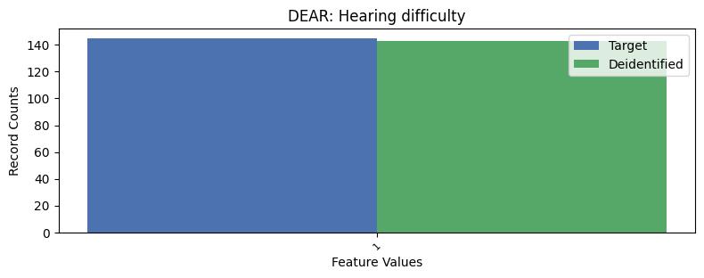
DEAR: Hearing difficulty:


Feature Value: 2
Target Data Counts: 26282
Deidentified Data Counts: 26357

DEAR

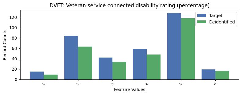
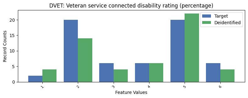
DVET: Veteran service connected disability rating (percentage):


Feature Value: N (N/A)
Target Data Counts: 26906
Deidentified Data Counts: 26965

DVET

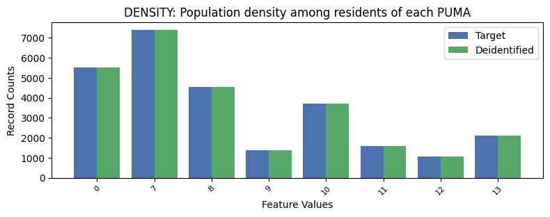
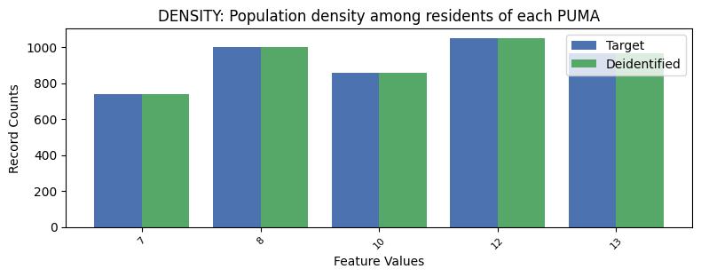
DENSITY: Population density among residents of each PUMA:


DENSITY

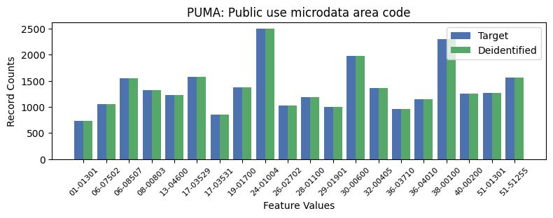
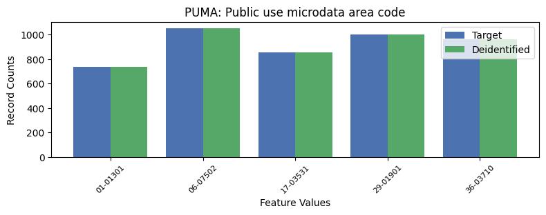
PUMA: Public use microdata area code:


PUMA


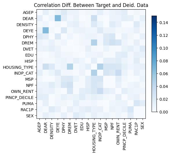
Correlations:


A key goal of deidentified data is to preserve the feature correlations from the target data, so that analyses performed on the deidentified data provide meaningful insight about the target population. Which correlations are the deidentified data preserving, and which are being altered during deidentification?

Kendall Tau Correlation Coefficient Difference:

This chart shows pairwise correlations using a somewhat different definition of correlation. To what extent do the two different correlation metrics agree or disagree with each other about the quality of the deidentified data?

corr_diff

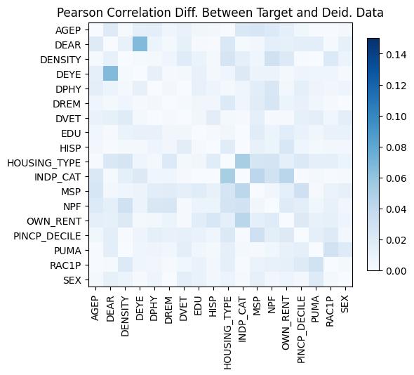
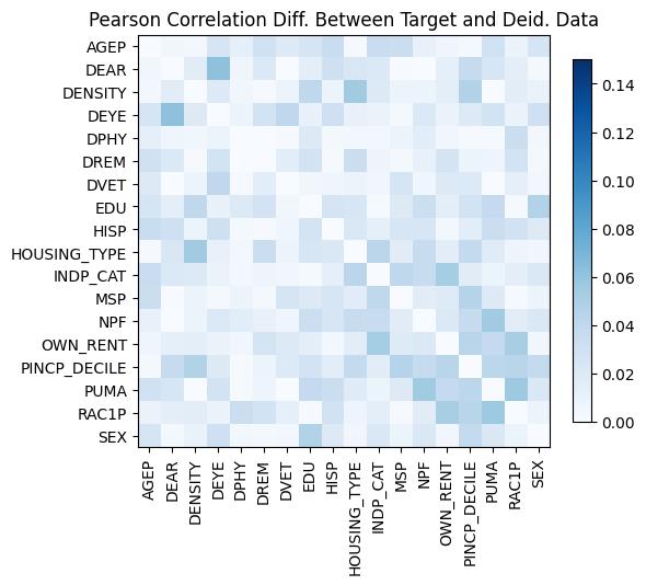
Pearson Correlation Coefficient Difference:

The Pearson Correlation difference was a popular utility metric during the HLG-MOS Synthetic Data Test Drive. Note that darker highlighting indicates pairs of features whose correlations were not well preserved by the deidentified data.

pearson_corr_diff


Linear Regression:


Linear regression is a fundamental data analysis technique that condenses a multi-dimensional data distribution down to a one dimensional (line) representation. It works by finding the line that sits in the 'middle' of the data, in some sense-- it minimizes the total distance between the points of the data and the line. There are more advanced forms of regression, but here we're focusing on the simplest case-- we fit a simple straight line to the data, getting the slope and y-intercept value of that line.

For this metric we're just looking at data from adults (AGEP > 15) and we're only considering the distribution of the data across two features:
  • EDU: The highest education level this individual has attained, ranging from 1 (elementary school) to 12 (PhD). See Appendix of this report for the full list of code values.
  • PINCP_DECILE: The individual's income decile relative to their PUMA. This helps us account for differences in cost of living across the country. If an individual makes a moderate income but lives in a very low income area, they may have a high value for PINCP_DECILE indicating that they have a high income for their PUMA).

The basic idea is that higher values of EDU should lead to higher values of PINCP_DECILE, and this is broadly true. However, it is known that the relationship between EDU and PINCP_DECILE is different for different demographic subgroups. The heatmaps in the left column below show the density distribution of the true data for each subgroup, normalized by education category (so the density values in each column sum to 1; note that when a cell in the heatmap contains too few people (< 20 ), it is left blank; its not expected that the deidentified data will match the original distribution precisely). The regression line is drawn in red over the heatmap, so you can see the relationship between the target data distribution and its linear regression analysis. In the right column for each subgroup we show how the deidentified data's regression line compares to the target data's regression line, along with a heatmap of the density differences between the two distributions. Redder areas are where the deidentified data has created too many people, bluer areas are where it's created too few people.

We've broken this metric down into demographic subgroups so we can see not only how well the privacy techniques preserve the overall relationship between these features, but also whether they preserve how that overall relationship is built up from the different relationships that hold at each major demographic subgroup. It's important that deidentification techniques preserve these distinct subgroup patterns for analysis.

Total Population:

Target Data:

23006 records, 100.0% of adult (>15) data
Regression: 0.63 slope, -0.1 intercept

Deidentified Data:

23080 records, 100.0% of adult (>15) data
Regression: 0.59 slope, 0.37 intercept
density_plot

White Men:

Target Data:

6463 records, 28.09% of adult (>15) data
Regression: 0.68 slope, 0.39 intercept

Deidentified Data:

6468 records, 28.02% of adult (>15) data
Regression: 0.63 slope, 0.8 intercept
density_plot

White Women:

Target Data:

6505 records, 28.28% of adult (>15) data
Regression: 0.66 slope, -0.6 intercept

Deidentified Data:

6666 records, 28.88% of adult (>15) data
Regression: 0.63 slope, -0.12 intercept
density_plot

Black Men:

Target Data:

2720 records, 11.82% of adult (>15) data
Regression: 0.52 slope, 0.45 intercept

Deidentified Data:

2652 records, 11.49% of adult (>15) data
Regression: 0.42 slope, 1.31 intercept
density_plot

Black Women:

Target Data:

3366 records, 14.63% of adult (>15) data
Regression: 0.51 slope, 0.3 intercept

Deidentified Data:

3288 records, 14.25% of adult (>15) data
Regression: 0.4 slope, 1.1 intercept
density_plot

Asian Men:

Target Data:

914 records, 3.97% of adult (>15) data
Regression: 0.7 slope, -0.68 intercept

Deidentified Data:

828 records, 3.59% of adult (>15) data
Regression: 0.72 slope, -0.25 intercept
density_plot

Asian Women:

Target Data:

982 records, 4.27% of adult (>15) data
Regression: 0.55 slope, -0.19 intercept

Deidentified Data:

892 records, 3.86% of adult (>15) data
Regression: 0.57 slope, -0.19 intercept
density_plot

American Indian, Alaskan Native and Native Hawaiians (AIANNH) Men:

Target Data:

376 records, 1.63% of adult (>15) data
Regression: 0.42 slope, 1.18 intercept

Deidentified Data:

368 records, 1.59% of adult (>15) data
Regression: 0.56 slope, 0.63 intercept
density_plot

American Indian, Alaskan Native and Native Hawaiians (AIANNH) Women:

Target Data:

395 records, 1.72% of adult (>15) data
Regression: 0.54 slope, -0.19 intercept

Deidentified Data:

466 records, 2.02% of adult (>15) data
Regression: 0.42 slope, 0.69 intercept
density_plot


Propensity Mean Square Error:


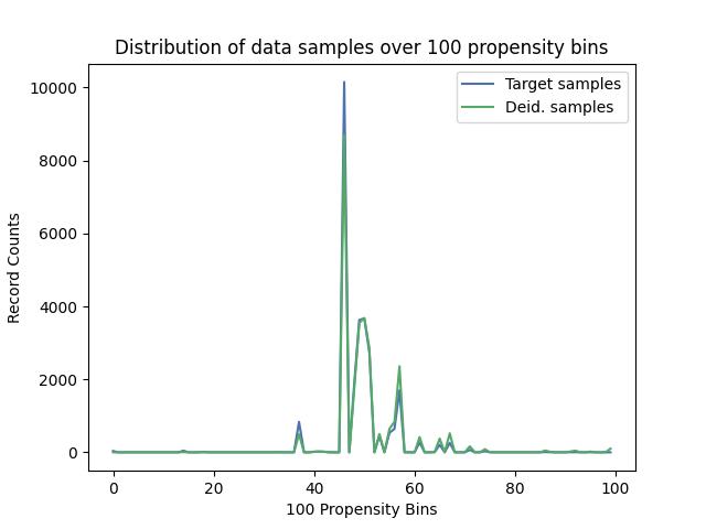
Can a decision tree classifier tell the difference between the target data and the deidentified data? If a classifier is trained to distinguish between the two data sets and it performs poorly on the task, then the deidentified data must not be easy to distinguish from the target data. If the green line matches the blue line, then the deidentified data is high quality. Propensity based metrics have been developed by Joshua Snoke and Gillian Raab and Claire Bowen, all of whom have participated on the NIST Synthetic Data Challenges SME panels.

Score: 0.004

Propensities Distribution:

propensity_distribution


PCA:


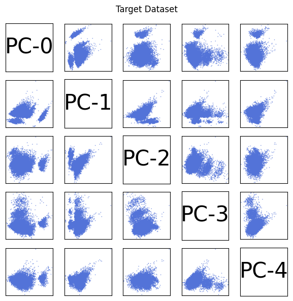
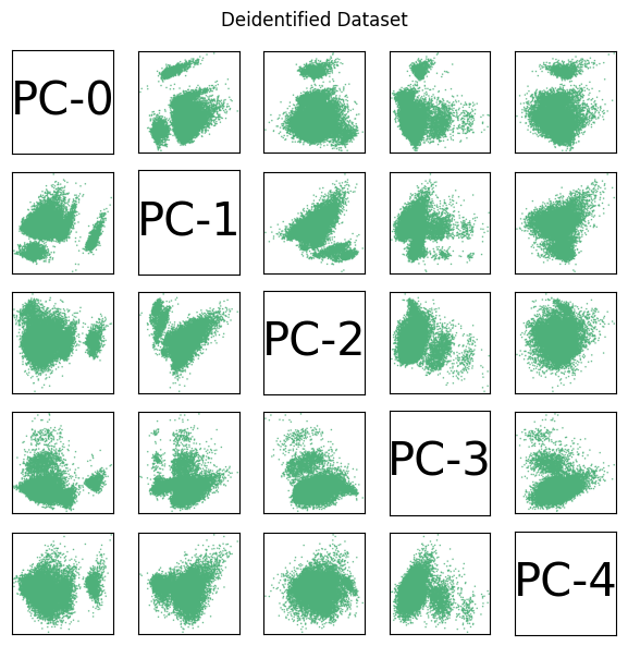
This is another approach for visualizing where the distribution of the deidentified data has shifted away from the target data. In this approach, we begin by using Principle Component Analysis to find a way of representing the target data in a lower dimensional space (in 5 dimensions rather than the full 22 dimensions of the original feature space). Descriptions of these new five dimensions (components) are given in the components table; the components will change depending on which target data set you’re using. Five dimensions are better than 22, but we actually want to get down to two dimensions so we can plot the data on simple (x,y) axes– the plots below show the data across each possible pair combination of our five components. You can compare how the shapes change between the target data and the deidentified data, and consider what that might mean in light of the component definitions. This is a relatively new visualization metric that was introduced by the IPUMS International team during the HLG-MOS Synthetic Data Test Drive.

Contribution of Features in Each Principal Component:

Principal Component Features Contribution: feature-name (contribution ratio)
PC-0 NPF (0.26),PWGTP (0.14),WGTP (0.14),OWN_RENT (0.12),RAC1P (0.09)
PC-1 WGTP (0.46),OWN_RENT (0.45),PWGTP (0.4),INDP_CAT (0.19),DPHY (0.16)
PC-2 HOUSING_TYPE (0.44),DENSITY (0.38),MSP (0.36),PWGTP (0.28),RAC1P (0.21)
PC-3 AGEP (0.29),DVET (0.2),MSP (0.17),PWGTP (0.17),WGTP (0.15)
PC-4 PWGTP (0.41),WGTP (0.38),POVPIP (0.35),DEYE (0.23),PINCP_DECILE (0.21)

target
deidentified

PCA Queries:


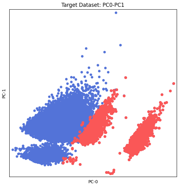
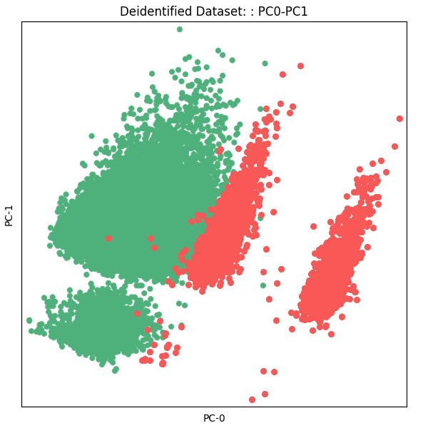
The queries below explore the PCA metric results in more detail by zooming in on a single component-pair panel and highlighting all individuals that satisfy a given constraint (such as MSP = “N”, individuals who are unmarried because they are children). If the deidentified data preserves the structure and feature correlations of the target data, the highlighted areas should have similar shape.

MSP_N: Children (AGEP < 15):


MSP_N
MSP_N


Inconsistencies:


Summary:

Inconsistency Group Number of Records Inconsistent Percent Records Inconsistent
Age 53 0.2%
Work 0 0.0%
Housing 5 0.0%

Age-Based Inconsistencies:

These inconsistencies deal with the AGE feature; records with age-based inconsistencies might have children who are married, or infants with high school diplomas

child_MSP: Children (< 15) can't be married:

12 violations

Example Record:

AGEP DEAR DENSITY DEYE DPHY DREM DVET EDU HISP HOUSING_TYPE INDP_CAT MSP NPF OWN_RENT PINCP_DECILE POVPIP PUMA PWGTP RAC1P SEX WGTP
10 2 7 2 2 2 N 7 0 3 14 6 N 0 1 N 13-04600 52 2 2 0

child_PINCP_DECILE: Children (< 15) don't have personal incomes:

12 violations

Example Record:

AGEP DEAR DENSITY DEYE DPHY DREM DVET EDU HISP HOUSING_TYPE INDP_CAT MSP NPF OWN_RENT PINCP_DECILE POVPIP PUMA PWGTP RAC1P SEX WGTP
10 2 7 2 2 2 N 7 0 3 14 6 N 0 1 N 13-04600 52 2 2 0

child_INDP_CAT: Children (< 15) don't have work industries:

12 violations

Example Record:

AGEP DEAR DENSITY DEYE DPHY DREM DVET EDU HISP HOUSING_TYPE INDP_CAT MSP NPF OWN_RENT PINCP_DECILE POVPIP PUMA PWGTP RAC1P SEX WGTP
9 2 7 2 2 2 N 3 0 2 4 N N 0 N N 13-04600 72 2 2 0

adult_N: Adults ( > 14) must specify values (other than N) for all adult features:

22 violations

Example Record:

AGEP DEAR DENSITY DEYE DPHY DREM DVET EDU HISP HOUSING_TYPE INDP_CAT MSP NPF OWN_RENT PINCP_DECILE POVPIP PUMA PWGTP RAC1P SEX WGTP
94 2 7 2 N N N N 0 1 N 3 2 1 2 54 01-01301 37 2 2 33

toddler_DPHY: Toddlers (< 5) naturally toddle, it's not a physical disability:

8 violations

Example Record:

AGEP DEAR DENSITY DEYE DPHY DREM DVET EDU HISP HOUSING_TYPE INDP_CAT MSP NPF OWN_RENT PINCP_DECILE POVPIP PUMA PWGTP RAC1P SEX WGTP
4 2 7 2 2 2 N 3 0 1 N N 3 2 N 231 13-04600 295 2 2 261

toddler_DREM: Toddlers (< 5) are naturally forgetful, it's not a cognitive disability:

10 violations

Example Record:

AGEP DEAR DENSITY DEYE DPHY DREM DVET EDU HISP HOUSING_TYPE INDP_CAT MSP NPF OWN_RENT PINCP_DECILE POVPIP PUMA PWGTP RAC1P SEX WGTP
4 2 7 2 2 2 N 3 0 1 N N 3 2 N 231 13-04600 295 2 2 261

infant_EDU: Infants (< 3) aren't in school:

1 violations

Example Record:

AGEP DEAR DENSITY DEYE DPHY DREM DVET EDU HISP HOUSING_TYPE INDP_CAT MSP NPF OWN_RENT PINCP_DECILE POVPIP PUMA PWGTP RAC1P SEX WGTP
2 2 7 2 N N N 1 0 1 N N 6 1 N 501 08-00803 44 1 1 52

Work-Based Inconsistencies:

These inconsistencies deal with the work and finance features; records with work-based inconsistencies might have high incomes while being in poverty, or have conflicts between their industry code and industry category.

Housing-Based Inconsistencies:

These inconsistencies deal with housing and family features; records with household-based inconsistencies might have more children in the house than the total household size, or be residents of group quarters (such as prison inmates) who are listed as owning their residences.

gq_h_family_NPF: Individuals who live in group quarters aren't considered family households:

3 violations

Example Record:

AGEP DEAR DENSITY DEYE DPHY DREM DVET EDU HISP HOUSING_TYPE INDP_CAT MSP NPF OWN_RENT PINCP_DECILE POVPIP PUMA PWGTP RAC1P SEX WGTP
72 2 8 2 1 2 N 3 4 2 N 1 2 0 3 N 24-01004 61 2 2 0

house_OWN_RENT: Individuals who live in houses must specify if they rent or own:

2 violations

Example Record:

AGEP DEAR DENSITY DEYE DPHY DREM DVET EDU HISP HOUSING_TYPE INDP_CAT MSP NPF OWN_RENT PINCP_DECILE POVPIP PUMA PWGTP RAC1P SEX WGTP
48 2 10 2 2 2 N 7 0 1 10 6 N 0 2 68 17-03531 198 2 1 198


K-Marginal Score Breakdown:


In the metrics above we’ve considered all of the data together; however we know that algorithms may behave differently on different subgroups in the population. Below we look in more detail at deidentification performance just in the worst performing PUMA, based on k-marginal score.

5 Worst Performing PUMA:

Which are the worst performing PUMA?

Record Counts in 5 Worst Performing PUMA:

Did the deidentified versions of these PUMA have similar population totals to the target versions?

Dataset Record Counts
Target 4608
Deidentified 4608

Univariate Distribution of Worst Performing Features in 5 Worst Performing PUMA:


Which features are performing the worst in each of these PUMA?

AGEP: Person's age:


AGEP

WGTP: Housing unit sampling weight:


WGTP

PWGTP: Person's sampling weight:


PWGTP

PINCP_DECILE: Person's total income in 10-percentile bins:


PINCP_DECILE

EDU: Educational attainment:


EDU

POVPIP: Income-to-poverty ratio (ex: 250 = 2.5 x poverty line):


Feature Value: 501 (Not in poverty: income above 5 x poverty line)
Target Data Counts: 1080
Deidentified Data Counts: 1148

POVPIP

INDP_CAT: Industry categories:


Feature Value: N (N/A)
Target Data Counts: 1963
Deidentified Data Counts: 1755

INDP_CAT

MSP: Marital Status:


MSP

RAC1P: Person's Race:


RAC1P

OWN_RENT: Housing unit rented or owned:


OWN_RENT

NPF: Number of persons in family (unweighted):


NPF

HISP: Hispanic origin:


Feature Value: 0
Target Data Counts: 3834
Deidentified Data Counts: 3699

HISP

DPHY: Ambulatory (walking) difficulty:


Feature Value: 2
Target Data Counts: 3874
Deidentified Data Counts: 3959

DPHY

HOUSING_TYPE: Housing unit or group quarters:


Feature Value: 1
Target Data Counts: 4167
Deidentified Data Counts: 4248

HOUSING_TYPE

SEX: Person's gender:


SEX

DEYE: Vision difficulty:


Feature Value: 2
Target Data Counts: 4438
Deidentified Data Counts: 4489

DEYE

DREM: Cognitive difficulty:


Feature Value: 2
Target Data Counts: 4050
Deidentified Data Counts: 4065

DREM

DENSITY: Population density among residents of each PUMA:


DENSITY

DVET: Veteran service connected disability rating (percentage):


Feature Value: N (N/A)
Target Data Counts: 4548
Deidentified Data Counts: 4554

DVET

DEAR: Hearing difficulty:


Feature Value: 2
Target Data Counts: 4463
Deidentified Data Counts: 4465

DEAR

PUMA: Public use microdata area code:


PUMA

Pearson Correlation Coefficient Difference in 5 Worst Performing PUMA:

How are feature correlations performing in each of these PUMA?

pearson_corr_diff

Privacy Evaluation

Apparent Match Distribution:


Quasi-Identifiers:

These features are used to determine if a deidentified record looks like it might be a real person in the target data.

SEX, EDU, RAC1P, INDP_CAT

Records Matched on Quasi-Identifiers:

Based only on the quasi-identifier features, how many deidentified records uniquely match an individual in the target data? What percentage of the deidentified data has apparent real matches?

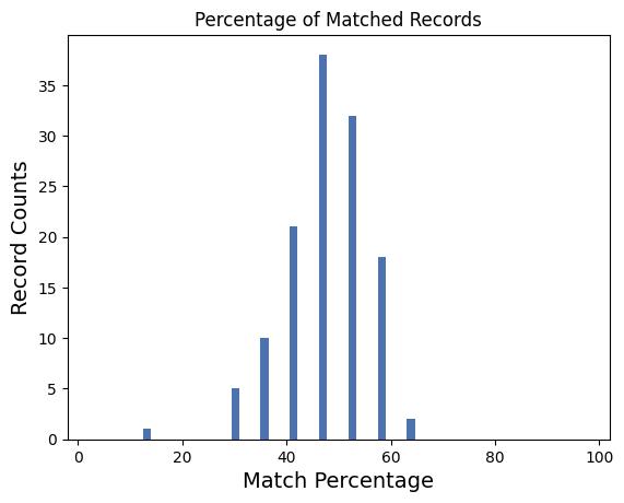
127, 0.005% of the deidentified records

Percentage Similarity of the Matched Records:

Considering the set of apparent matches, to what extent are they real matches? This distribution shows edit similarity between apparently matched pairs on how many of the 22 features does the deidentified record have the same value as the real record. If the distribution is centered near 100% that means these deidentified records largely mimic target records and are potentially leaking information about real individuals. If the distribution is centered below 50% that means the deidentified records are very different from the target records, and the apparent matches are not real matches.

apparent_match_distribution

Appendix

Data Dictionary:


PUMA: Public use microdata area code:

PUMA Code Code Description
25-00503 Middlesex County--Waltham City, Lexington, Burlington, Bedford & Lincoln Towns
25-00703 Essex County (East)--Salem, Beverly, Gloucester & Newburyport Cities
25-01000 Peabody City, Danvers, Reading, North Reading & Lynnfield Towns
25-01300 Billerica, Andover, Tewksbury & Wilmington Towns
25-02800 Woburn, Melrose Cities, Saugus, Wakefield & Stoneham Towns
48-02510 Tarrant County (North)--North Richland Hills (North) & Keller Cities
48-02102 Johnson County
48-02101 Ellis County
48-02515 Tarrant County (West)--Fort Worth City (West)
48-02507 Tarrant County (East)--Arlington City (West)--South of I-30 & East of Loop I-820
48-02516 Tarrant County (Southwest)--Fort Worth (Southwest) & Benbrook Cities
01-01301 Birmingham City (West)
06-07502 San Francisco County (North & East)--North Beach & Chinatown
06-08507 Santa Clara County (Southwest)--Cupertino, Saratoga Cities & Los Gatos Town
08-00803 Boulder County (Central)--Boulder City
13-04600 Atlanta Regional Commission--Fulton County (Central)--Atlanta City (Central)
17-03529 Chicago City (South)--South Shore, Hyde Park, Woodlawn, Grand Boulevard & Douglas
17-03531 Chicago City (South)--Auburn Gresham, Roseland, Chatham, Avalon Park & Burnside
19-01700 Des Moines City
24-01004 Montgomery County (South)--Bethesda, Potomac & North Bethesda
26-02702 Washtenaw County (East Central)--Ann Arbor City Area
28-01100 Central Region--Jackson City (East & Central)
29-01901 St. Louis City (North)
30-00600 East Montana (Outside Billings City)
32-00405 Las Vegas City (Southeast)
36-03710 NYC-Bronx Community District 1 & 2--Hunts Point, Longwood & Melrose
36-04010 NYC-Brooklyn Community District 17--East Flatbush, Farragut & Rugby
38-00100 West North Dakota--Minot City
40-00200 Cherokee, Sequoyah & Adair Counties
51-01301 Arlington County (North)
51-51255 Alexandria City

AGEP: Person's age:

AGEP Code Code Description
min 0
max 99

SEX: Person's gender:

SEX Code Code Description
1 Male
2 Female

MSP: Marital Status:

MSP Code Code Description
N N/A (age less than 15 years)
1 Now married, spouse present
2 Now Married, spouse absent
3 Widowed
4 Divorced
5 Separated
6 Never married

HISP: Hispanic origin:

HISP Code Code Description
0 Not Spanish/Hispanic/Latino
1 Mexican
2 Puerto Rican
3 Cuban
4 All other Spanish/Hispanic/Latino

RAC1P: Person's Race:

RAC1P Code Code Description
1 White alone
2 Black or African American alone
3 American Indian alone
4 Alaska Native alone
5 American Indian and Alaska Native tribes specified; or American Indian or Alaska Native, not specified and no other races
6 Asian alone
7 Native Hawaiian and Other Pacific Islander alone
8 Some Other Race alone
9 Two or More Races

NOC: Number of own children in household (unweighted):

NOC Code Code Description
N N/A (GQ/vacant)
0 No own children
min 1
max 19

NPF: Number of persons in family (unweighted):

NPF Code Code Description
N N/A (GQ/vacant/non-family household
min 2
max 20

HOUSING_TYPE: Housing unit or group quarters:

HOUSING_TYPE Code Code Description
1 Housing Unit
2 Institutional Group Quarters
3 Non-institutional Group Quarters

OWN_RENT: Housing unit rented or owned:

OWN_RENT Code Code Description
0 Group quarters
1 Own housing unit
2 Rent housing unit

DENSITY: Population density among residents of each PUMA:

DENSITY Code Code Description
min 16.3
max 52864.7

Density Bin: 0 | Bin Range: (0, 150]
PUMA DENSITY PUMA NAME
30-00600 16.0 East Montana (Outside Billings City)
38-00100 73.0 West North Dakota--Minot City
40-00200 90.0 Cherokee, Sequoyah & Adair Counties

Density Bin: 7 | Bin Range: (2646.76, 4065.16]
PUMA DENSITY PUMA NAME
01-01301 2731.0 Birmingham City (West)
06-08507 3305.0 Santa Clara County (Southwest)--Cupertino, Saratoga Cities & Los Gatos Town
08-00803 3393.0 Boulder County (Central)--Boulder City
13-04600 3670.0 Atlanta Regional Commission--Fulton County (Central)--Atlanta City (Central)
19-01700 3572.0 Des Moines City
28-01100 2674.0 Central Region--Jackson City (East & Central)

Density Bin: 8 | Bin Range: (4065.16, 6243.68]

PUMA DENSITY PUMA NAME
24-01004 4187.0 Montgomery County (South)--Bethesda, Potomac & North Bethesda
26-02702 4817.0 Washtenaw County (East Central)--Ann Arbor City Area
29-01901 5434.0 St. Louis City (North)

Density Bin: 9 | Bin Range: (6243.68, 9589.66]

PUMA DENSITY PUMA NAME
32-00405 7990.0 Las Vegas City (Southeast)

Density Bin: 10 | Bin Range: (9589.66, 14728.75]

PUMA DENSITY PUMA NAME
17-03531 11171.0 Chicago City (South)--Auburn Gresham, Roseland, Chatham, Avalon Park & Burnside
51-01301 11162.0 Arlington County (North)
51-51255 11224.0 Alexandria City

Density Bin: 11 | Bin Range: (14728.75, 22621.88]

PUMA DENSITY PUMA NAME
17-03529 15097.0 Chicago City (South)--South Shore, Hyde Park, Woodlawn, Grand Boulevard & Douglas

Density Bin: 12 | Bin Range: (22621.88, 34744.92]

PUMA DENSITY PUMA NAME
06-07502 33632.0 San Francisco County (North & East)--North Beach & Chinatown

Density Bin: 13 | Bin Range: (34744.92, 53364.7]

PUMA DENSITY PUMA NAME
36-03710 52864.0 NYC-Bronx Community District 1 & 2--Hunts Point, Longwood & Melrose
36-04010 50441.0 NYC-Brooklyn Community District 17--East Flatbush, Farragut & Rugby

INDP: Industry codes:

See codes in ACS data dictionary. Find codes by searching the string: INDP, in the ACS data dictionary

INDP_CAT: Industry categories:

INDP_CAT Code Code Description
N N/A (less than 16 years old/NILF who last worked more than 5 years ago or never worked)
0 AGR: Agriculture, Forestry, Fishing and Hunting
1 EXT: Mining, Quarrying, and Oil and Gas Extraction
2 UTL: Utilities
3 CON: Construction
4 MFG: Manufacturing
5 WHL: Wholesale Trade
6 RET: Retail Trade
7 TRN: Transportation and Warehousing
8 INF: Information
9 FIN: Finance, Insurance, Real Estate
10 PRF: Professional, Scientific and Technical Services
11 EDU: Educational Services
12 MED: Health Care
13 SCA: Social Assistance
14 ENT: Arts, Entertainment, Accommodation, Food Services and Recreation
15 SRV: Other Services
16 ADM: Government, Public Administration
17 MIL: Military
18 UNEMPLOYED

EDU: Educational attainment:

EDU Code Code Description
N N/A (less than 3 years old)
1 No schooling completed
2 Nursery school, Preschool, or Kindergarten
3 Grade 4 to grade 8
4 Grade 9 to grade 12, no diploma
5 High School diploma
6 GED
7 Some College, no degree
8 Associate degree
9 Bachelors degree
10 Masters degree
11 Professional degree
12 Doctorate degree

PINCP: Person's total income in dollars:

PINCP Code Code Description
N N/A (less than 15 years old)
min -9000
max 1341000

PINCP_DECILE: Person's total income in 10-percentile bins:

PINCP_DECILE Code Code Description
N N/A (less than 15 years old
9 90th percentile
8 80th percentile
7 70th percentile
6 60th percentile
5 50th percentile
4 40th percentile
3 30th percentile
2 20th percentile
1 10th percentile
0 0th percentile

POVPIP: Income-to-poverty ratio (ex: 250 = 2.5 x poverty line):

POVPIP Code Code Description
N N/A
min 0
max 500
501 income above 5 x poverty line

DVET: Veteran service connected disability rating (percentage):

DVET Code Code Description
N N/A (No service-connected disability/never served in military
1 0 percent
2 10 or 20 percent
3 30 or 40 percent
4 50 or 60 percent
5 70, 80, 90 or 100 percent
6 Not reported

DREM: Cognitive difficulty:

DREM Code Code Description
N N/A (Less than 5 years old)
1 Yes
2 No

DPHY: Ambulatory (walking) difficulty:

DPHY Code Code Description
N N/A (Less than 5 years old)
1 Yes
2 No

DEYE: Vision difficulty:

DEYE Code Code Description
1 Yes
2 No

DEAR: Hearing difficulty:

DEAR Code Code Description
1 Yes
2 No

WGTP: Housing unit sampling weight:

See description of weights.

WGTP Code Code Description
0 Group quarters place holder record
min 1
max 9999

PWGTP: Person's sampling weight:

See description of weights.

PWGTP Code Code Description
min 1
max 9999