Report created on: March 15, 2023 21:45:38
Created with SDNIST v2.1.0
Data Description
Deidentified (Deid.) Data:
| Label Name | Label Value |
|---|---|
| Team | CCAIM |
| Submission Timestamp | 3/9/2023 3:29:17 |
| Algorithm Name | Synthcity-PATEGAN |
| Variant Label | syntheticy-pategan-default |
| Property | Value |
|---|---|
| Filename | pategan-ZhaozhiQian |
| Records | 21802 |
| Features | 24 |
Target Data:
| Property | Value |
|---|---|
| Filename | national2019 |
| Records | 27253 |
| Features | 24 |
Evaluated Data Features:
| Feature Name | Feature Description | Feature Type | Feature Has 'N' (N/A) values? |
|---|---|---|---|
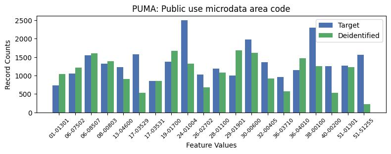
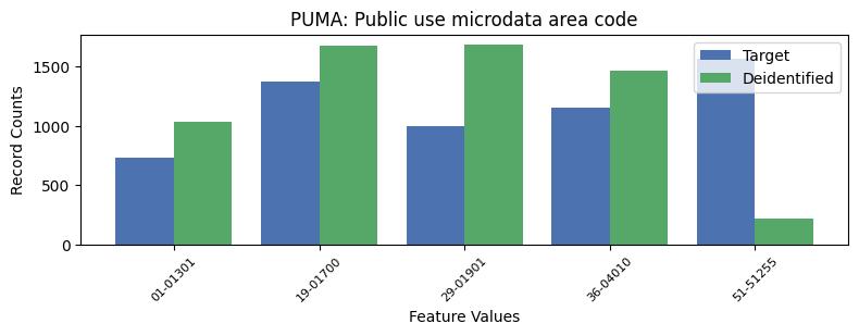
| PUMA | Public use microdata area code | object of type string | False |
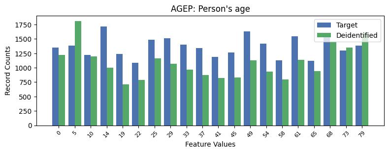
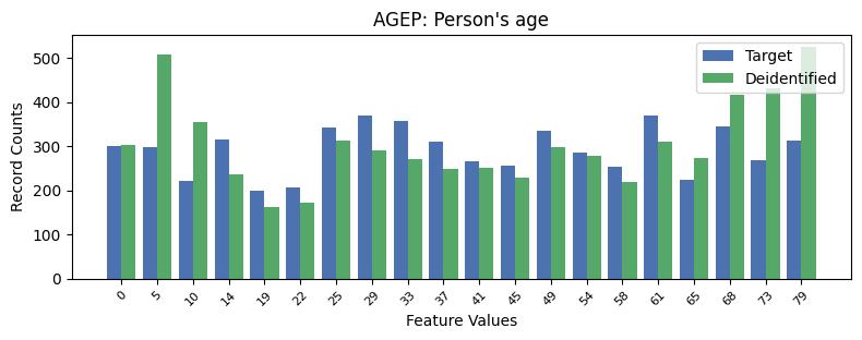
| AGEP | Person's age | int64 | False |
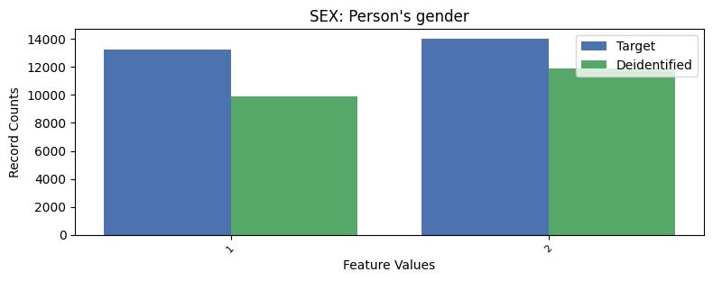
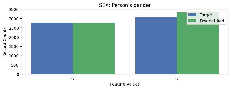
| SEX | Person's gender | int64 | False |
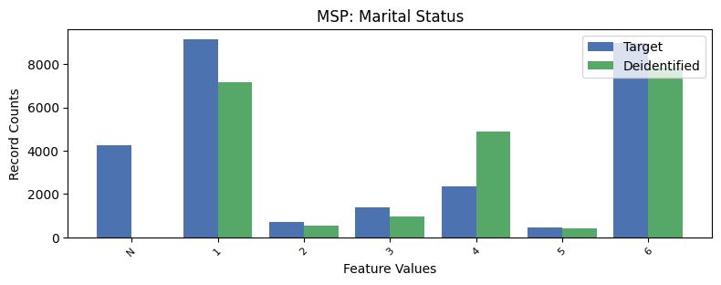
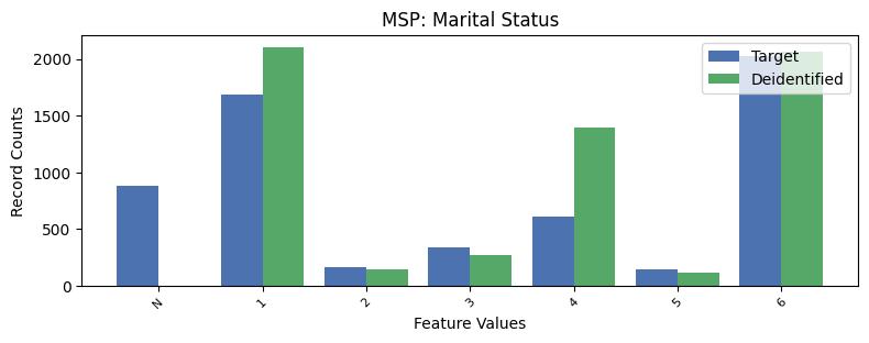
| MSP | Marital Status | object of type string | True |
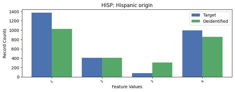
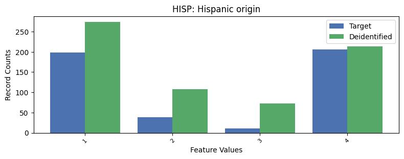
| HISP | Hispanic origin | int64 | False |
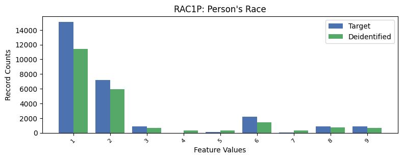
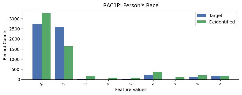
| RAC1P | Person's Race | int64 | False |
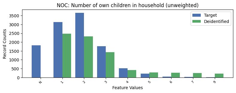
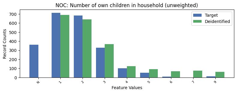
| NOC | Number of own children in household (unweighted) | object of type string | True |
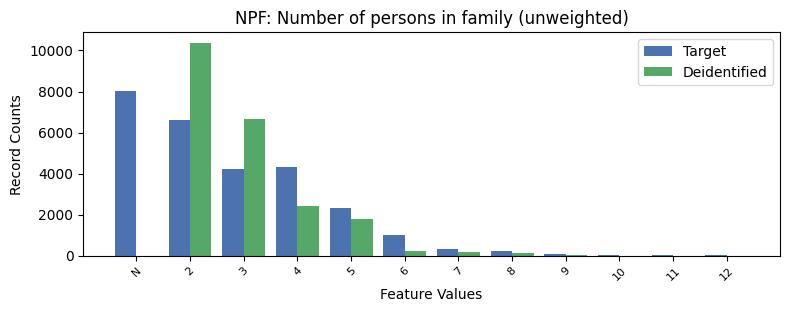
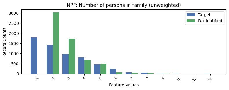
| NPF | Number of persons in family (unweighted) | object of type string | True |
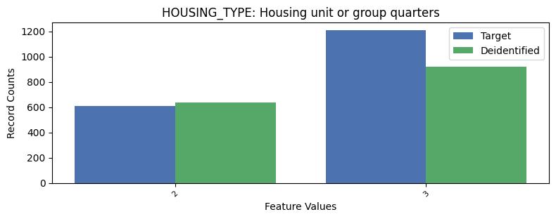
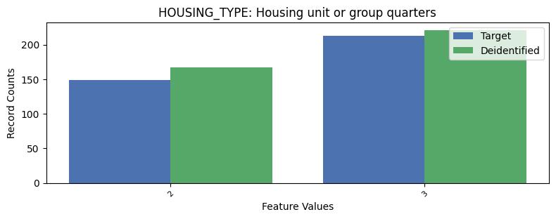
| HOUSING_TYPE | Housing unit or group quarters | int64 | False |
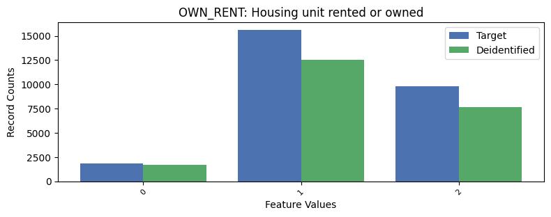
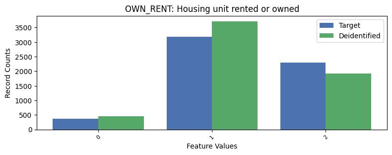
| OWN_RENT | Housing unit rented or owned | int64 | False |
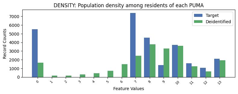
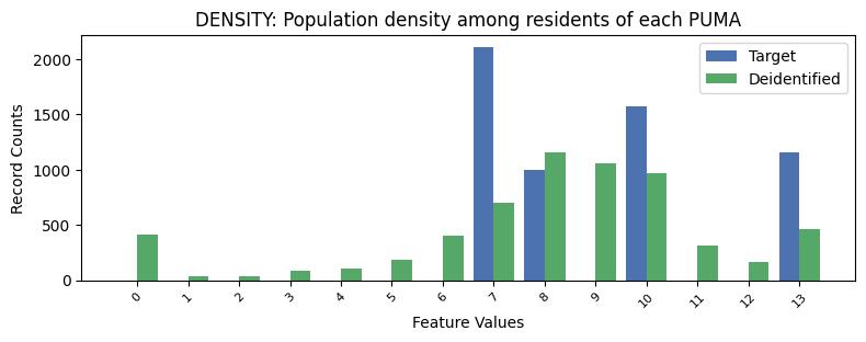
| DENSITY | Population density among residents of each PUMA | float64 | False |
| INDP | Industry codes | object of type string | True |
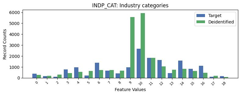
| INDP_CAT | Industry categories | object of type string | True |
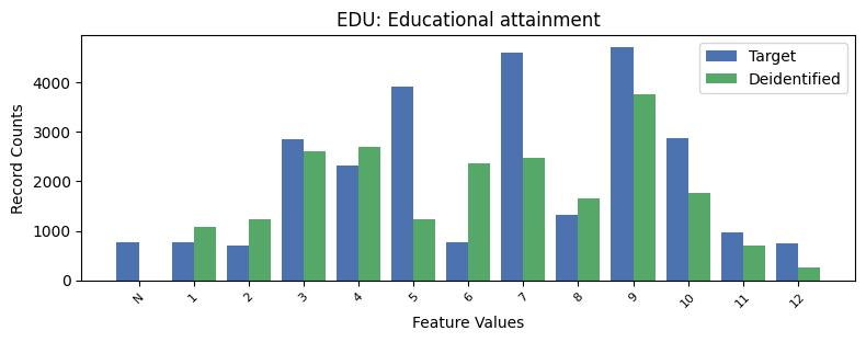
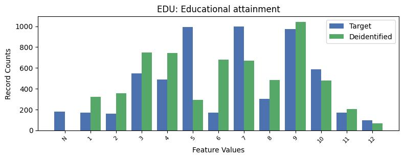
| EDU | Educational attainment | object of type string | True |
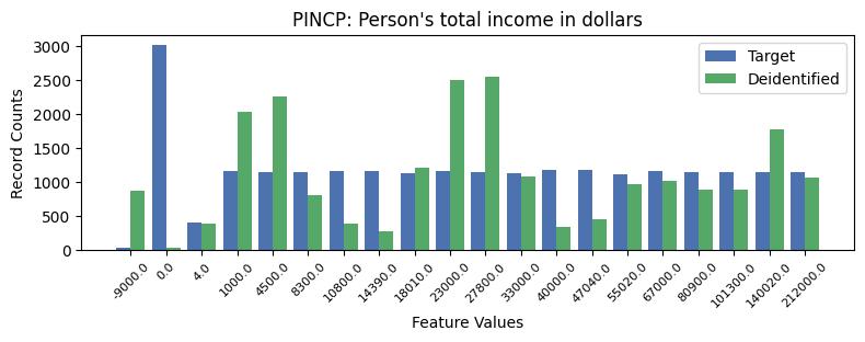
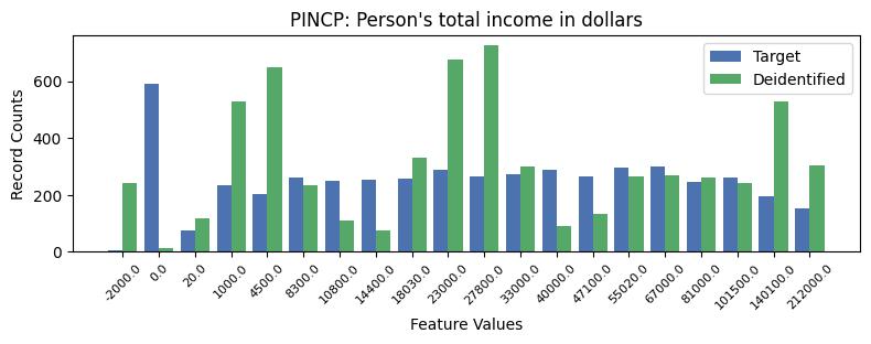
| PINCP | Person's total income in dollars | object of type string | True |
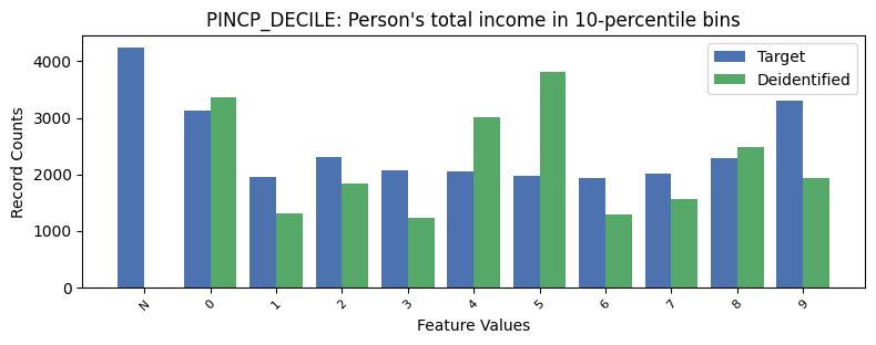
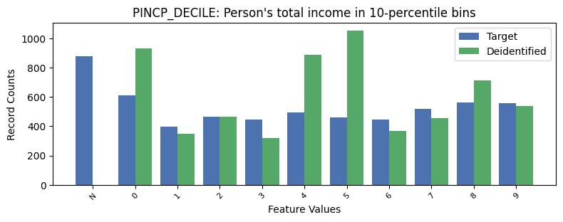
| PINCP_DECILE | Person's total income in 10-percentile bins | object of type string | True |
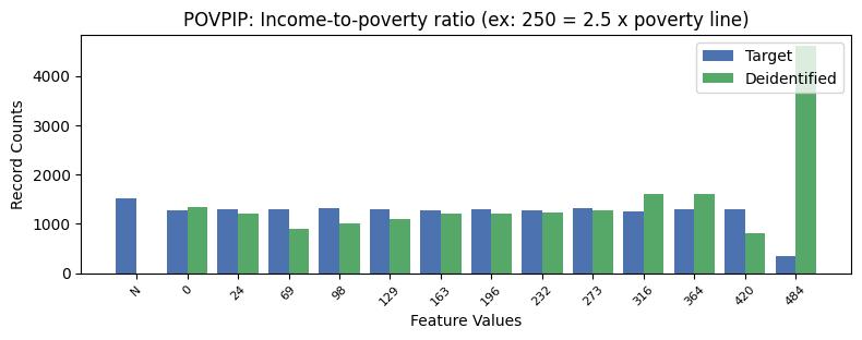
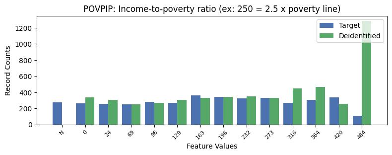
| POVPIP | Income-to-poverty ratio (ex: 250 = 2.5 x poverty line) | object of type string | True |
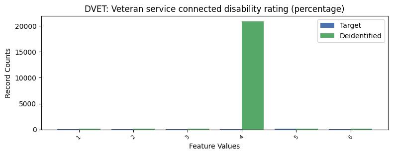
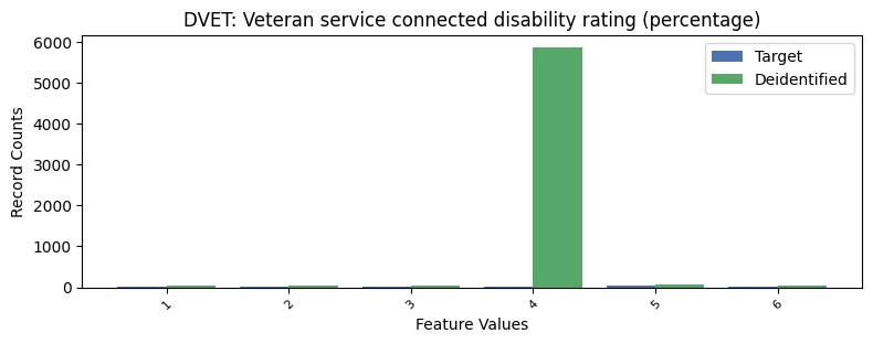
| DVET | Veteran service connected disability rating (percentage) | object of type string | True |
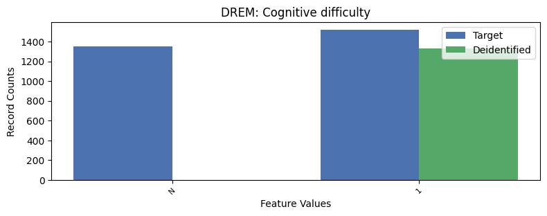
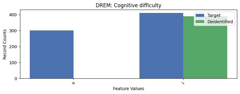
| DREM | Cognitive difficulty | object of type string | True |
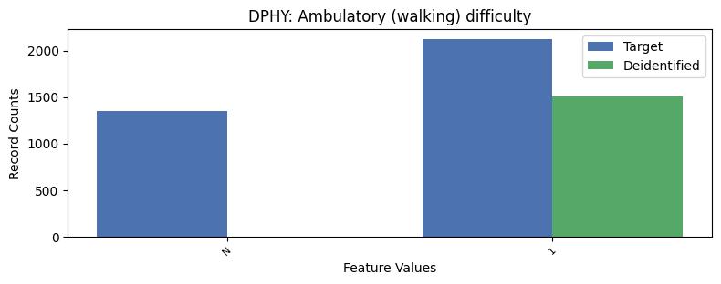
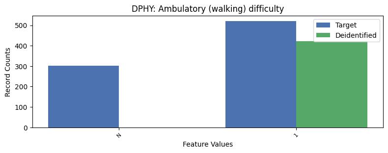
| DPHY | Ambulatory (walking) difficulty | object of type string | True |
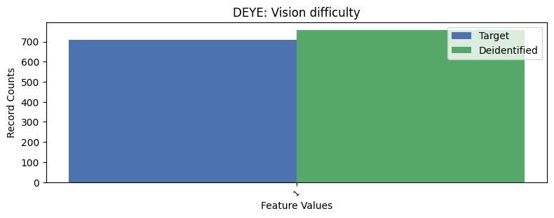
| DEYE | Vision difficulty | int32 | False |
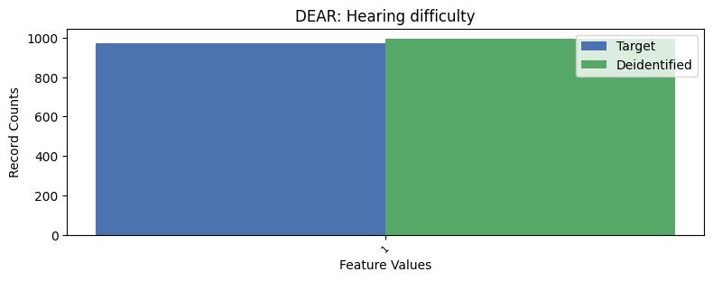
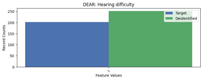
| DEAR | Hearing difficulty | int32 | False |
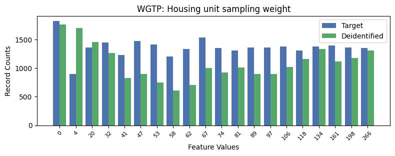
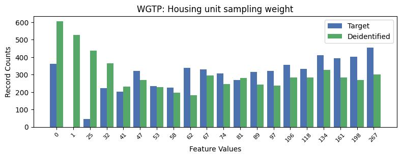
| WGTP | Housing unit sampling weight | int64 | False |
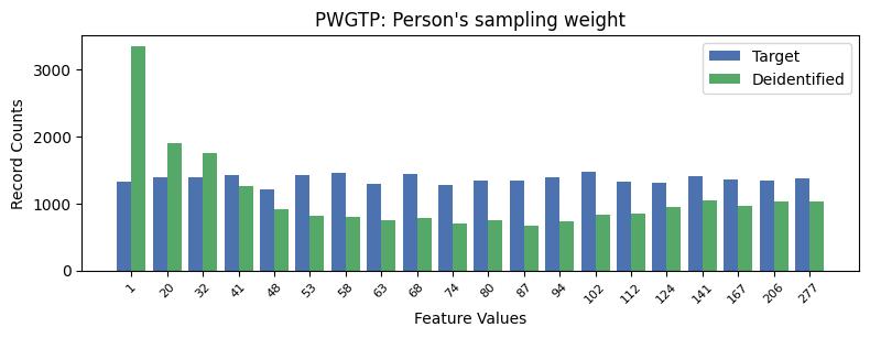
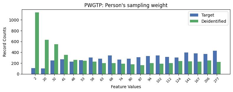
| PWGTP | Person's sampling weight | int64 | False |
Utility Evaluation
K-Marginal Synopsys:
Univariate Distributions:
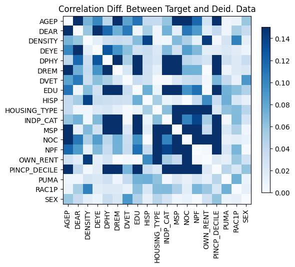
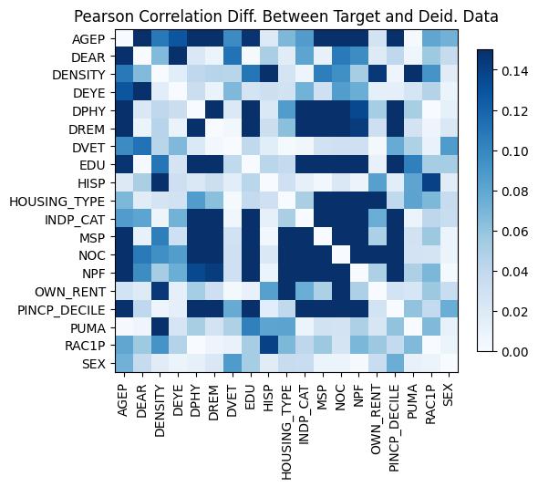
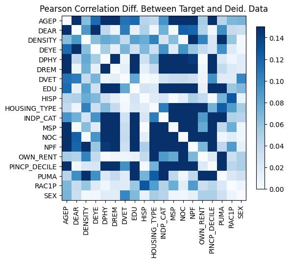
Correlations:
Linear Regression:
Total Population:
Target Data:
23006 records, 100.0% of adult (>15) data
Regression: 0.63 slope, -0.1 intercept
Deidentified Data:
21802 records, 100.0% of adult (>15) data
Regression: 0.32 slope, 2.38 intercept

White Men:
Target Data:
6463 records, 28.09% of adult (>15) data
Regression: 0.68 slope, 0.39 intercept
Deidentified Data:
5289 records, 24.26% of adult (>15) data
Regression: 0.36 slope, 2.41 intercept

White Women:
Target Data:
6505 records, 28.28% of adult (>15) data
Regression: 0.66 slope, -0.6 intercept
Deidentified Data:
6133 records, 28.13% of adult (>15) data
Regression: 0.35 slope, 2.6 intercept

Black Men:
Target Data:
2720 records, 11.82% of adult (>15) data
Regression: 0.52 slope, 0.45 intercept
Deidentified Data:
2646 records, 12.14% of adult (>15) data
Regression: 0.25 slope, 2.35 intercept

Black Women:
Target Data:
3366 records, 14.63% of adult (>15) data
Regression: 0.51 slope, 0.3 intercept
Deidentified Data:
3323 records, 15.24% of adult (>15) data
Regression: 0.25 slope, 2.24 intercept

Asian Men:
Target Data:
914 records, 3.97% of adult (>15) data
Regression: 0.7 slope, -0.68 intercept
Deidentified Data:
643 records, 2.95% of adult (>15) data
Regression: 0.3 slope, 2.58 intercept

Asian Women:
Target Data:
982 records, 4.27% of adult (>15) data
Regression: 0.55 slope, -0.19 intercept
Deidentified Data:
782 records, 3.59% of adult (>15) data
Regression: 0.3 slope, 2.43 intercept

American Indian, Alaskan Native and Native Hawaiians (AIANNH) Men:
Target Data:
376 records, 1.63% of adult (>15) data
Regression: 0.42 slope, 1.18 intercept
Deidentified Data:
675 records, 3.1% of adult (>15) data
Regression: 0.26 slope, 2.51 intercept

American Indian, Alaskan Native and Native Hawaiians (AIANNH) Women:
Target Data:
395 records, 1.72% of adult (>15) data
Regression: 0.54 slope, -0.19 intercept
Deidentified Data:
909 records, 4.17% of adult (>15) data
Regression: 0.14 slope, 3.1 intercept

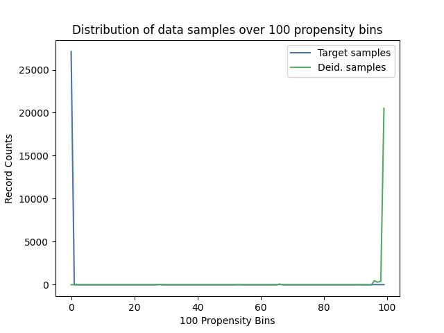
Propensity Mean Square Error:
Propensities Distribution:
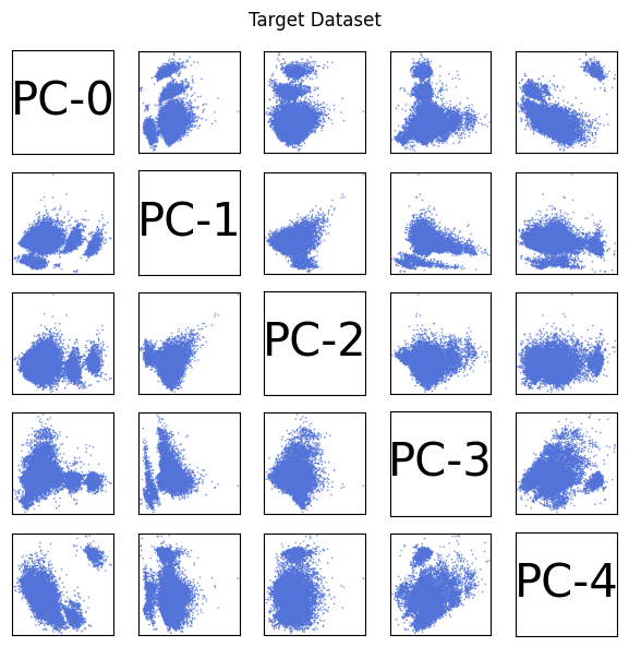
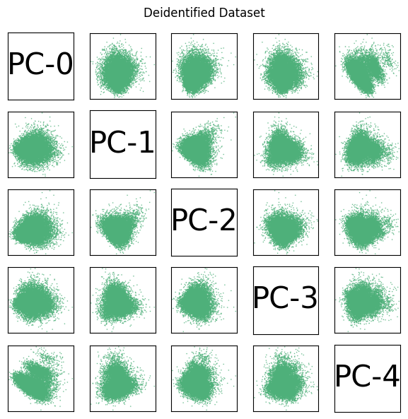
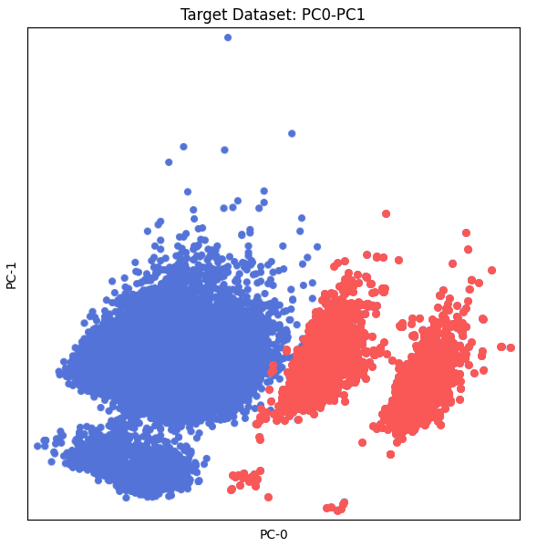
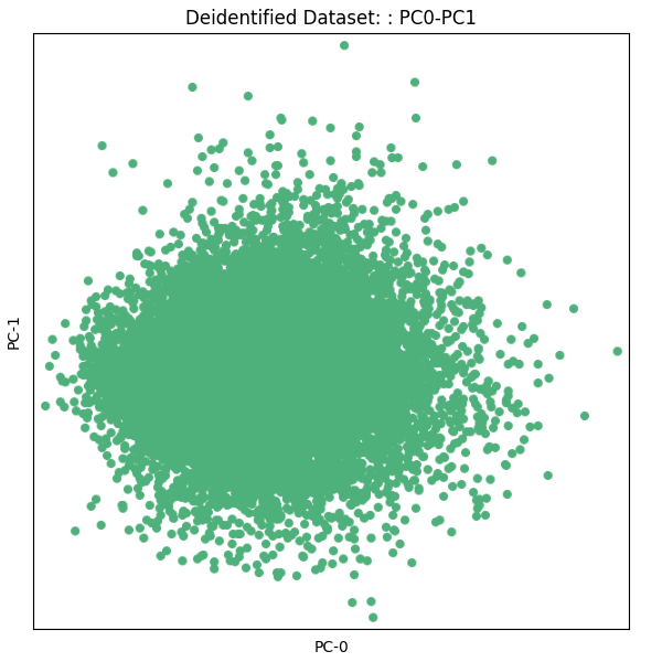
PCA:
Inconsistencies:
K-Marginal Score Breakdown:

Privacy Evaluation
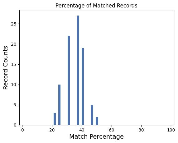
Apparent Match Distribution: