Benchmark Problem 6: Electrostatics¶

See the Overleaf document entitled "Phase Field Benchmark Problems for Dendritic Growth and Linear Elasticity" for more details about the benchmark problems. Furthermore, read the extended essay for a discussion about the need for benchmark problems.

Overview¶

Diffusion of a charged species is often modeled with the phase field approach, such as for batteries, electrodeposition, and electromigration. This benchmark problem incorporates the first benchmark problem for spinodal decomposition Jokisaari 2017 and extends it to incorporate coupling with electrostatics.

Governing Equations¶

In this problem, two variables are used: $c$, the concentration field of our charged species, and $\Phi$, the electric potential field. The free energy of the system is given as

\begin{equation} F=\int_{V} \left[\frac{\kappa}{2} |\nabla c|^2+f_{chem}(c)+f_{elec}(c,\Phi)\right]\,dV, \end{equation}

where $\kappa$ is the gradient energy coefficient, $f_{chem}$ is the chemical free energy, and $f_{elec}$ is the electrostatic coupling energy. Here, $f_{chem}$ is a symmetric double-well function with minima between $0<c<1$,

\begin{equation} f_{chem} = \rho (c-c^{\alpha})^2(c^{\beta}-c)^2, \end{equation}

where $\rho$ controls the height of the double-well and $c^{\alpha}$ and $c^{\beta}$ are the compositions at which the energy is minimum. In addition, the electrostatic coupling energy is given as

\begin{equation} f_{elec}=\frac{k\, c \, \Phi}{2}, \end{equation}

where $k$ is a constant.

The time evolution of the system is described by the Cahn-Hilliard equation with the additional constraint that the Poisson equation must be satisfied at every point in the system at each time step (Guyer 2004a, Guyer 2004b). To avoid a lengthy derivation, we simply present the equations below and suggest the readers study the given references. The Cahn-Hillard equation is given as

\begin{equation} \frac{\partial c}{\partial t} = \nabla \cdot \left\lbrace M \nabla \left( 2 \rho(c-c^{\alpha})(c^{\beta}-c)(c^{\alpha}+c^{\beta}-2c) -\kappa \nabla^2 c + k \, \Phi \right) \right\rbrace, \end{equation}

where $M$ is the mobility. The dynamics of electric relaxation occur at a much faster time scale than the diffusion of the charged species. In this case, the Poisson equation is solved at each time step,

\begin{equation} \nabla^2 \Phi = \frac{-k\, c}{\epsilon}, \end{equation}

where $\epsilon$ is the permittivity.

As in the spinodal benchmark problem, $c^{\alpha}=0.3$, $c^{\beta}=0.7$, $\kappa=2$, $\rho=5$, and $M=5$. In addition, $k=0.09$ and $\epsilon=90$.

Domain¶

In this problem, the system consists of a domain which is grounded on one side and with a voltage applied on the other. Two different 2D computational domains are given, shown below (the boundary conditions for $\Phi$ are schematically illustrated). The first consists of a square domain, while the second consists of a half-circle with a radius of 50 units and centered at (50, 50), which is attached to a rectangle of 50 units wide by 100 units tall. The curved boundary is the right-hand boundary, while the straight domain edges from (0, 0) to (50, 0) and (0, 100) to (50, 100) are the bottom and top boundaries, respectively. Schematic illustrations of the 2D computational domains and boundary conditions of $\Phi$ (indicated by hatching) for the electrochemical benchmark problem are shown in Figures 1 and 2.

Figure 1: Domain (a)¶

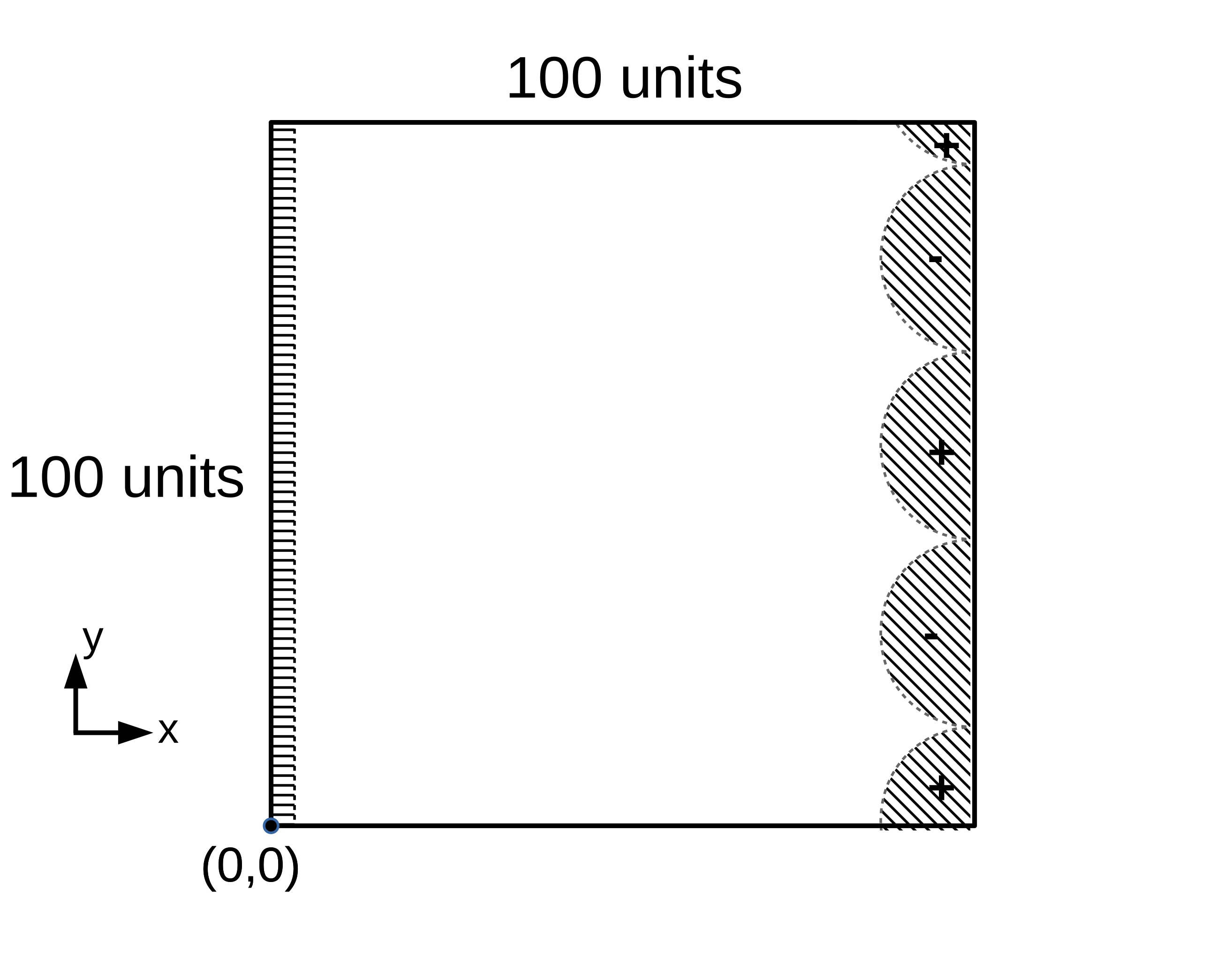
Figure 2: Domain (b)¶

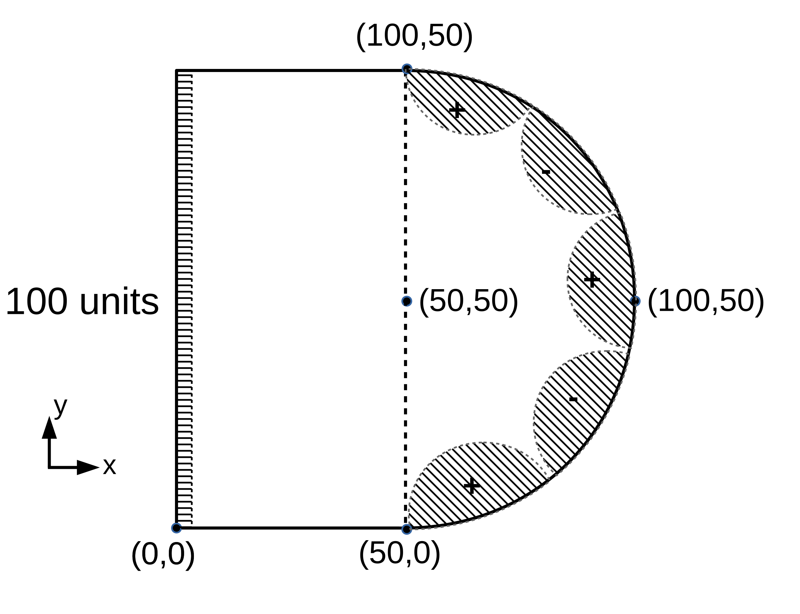
Boundary Conditions¶

We impose no-flux boundary conditions on all boundaries, while $\Phi=0$ for the left boundary, $\nabla \Phi \cdot \hat{\textbf{n}}=0$ for the top and bottom boundaries, and the right boundary is given by

\begin{equation} \Phi(x|_{boundary},y) = \sin(y/7), \end{equation}

where $x|_{boundary}=100$ for domain (a), and varies from 50 to 100 in domain (b). The initial condition for $c$ is specified by

\begin{eqnarray} c\left(x,y\right) & = & c_{0}+c_{1}\left\{\cos\left(0.2x\right)\cos\left(0.11y\right)+\left[\cos\left(0.13x\right)\cos\left(0.087y\right)\right]^{2}\right. \\ & & \left.+\cos\left(0.025x-0.15y\right)\cos\left(0.07x-0.02y\right)\right\}, \end{eqnarray}

where $c_{0}=0.5$ and $c_{1}=0.04$ (you may recognize this as the initial conditions for the spinodal decomposition benchmark problem with a slightly different parameterization).

Submission Guidelines¶

Both variations (a) and (b) should be run for 400 time units. The following data should be collected from each simulation,

• the free energy integrated across the entire domain, $F$, collected as frequently as is feasible.

• the $c$ and $\Phi$ at $t=400$ along the $x=50$ cut plane

• the $c$ and $\Phi$ at $t=400$ along the $y=50$ cut plane

Thus each submission requires three data files for each variation,

• a CSV or JSON upload labeled as free_energy with column titles of time and free_energy

• a CSV or JSON upload labeled as x_cut_plane with column titles of y, concentration and potential

• a CSV or JSON upload labeled as y_cut_plane with column titles of x, concentration and potential

Further data to upload can include images of $c$ and $\Phi$ at different times or youtube videos of the evolution. These are not required, but will help others view your work.