from IPython.display import HTML

HTML('''<script>
code_show=true;
function code_toggle() {
 if (code_show){
 $('div.input').hide();
 $('div.prompt').hide();
 } else {
 $('div.input').show();
$('div.prompt').show();
 }
 code_show = !code_show
}
$( document ).ready(code_toggle);
</script>
<form action="javascript:code_toggle()"><input type="submit" value="Code Toggle"></form>''')
from IPython.display import HTML

HTML('''
<a href="https://github.com/usnistgov/pfhub/raw/master/benchmarks/benchmark3.ipynb"
   download="benchmark3.ipynb">
<button type="submit">Download Notebook</button>
</a>''')
Benchmark Problem 3: Dendritic Growth
from IPython.display import HTML

HTML('''{% include jupyter_benchmark_table.html num="[3]" revision=1 %}''')
See the journal publication entitled "Phase Field Benchmark Problems for Dendritic Growth and Linear Elasticity" for more details about the benchmark problems. Furthermore, read the extended essay for a discussion about the need for benchmark problems.
Overview
Dendritic growth simulations are useful as benchmark problems being highly sensitive to both the phase field model formulation and the particular numerical implementation employed (see, for example, [1, 2]). Historically, dendritic growth was one of the first applications of phase field modeling [3, 4], and remains a significant area of research today. Previous analyses of both the sharp [4, 5, 6, 7, 8] and thin interface limits [10, 1, 11, 12] have demonstrated that the diffuse-interface phase field formulation is asymptotically equivalent to the sharp-interface Stefan formulation. In 2001, the introduction of an "anti-trapping current" to correct for solute trapping due to the jump in chemical potential at the solid/liquid interface [13, 14] facilitated quantitative phase field modeling of alloy solidification using unphysically large diffuse interface widths. Today, massive increases in computing power and the advent of scientific computing on graphical processing units enable large-scale, quantitative 3D phase field simulations of growing dendrites (see, for example, [15, 16] and reviews [17, 18]).
Model Formulation
In this formulation, one order parameter, $\phi$, and one additional field variable, $U$, are evolved. The phase of the material is described by $\phi$, which takes a value of -1 in the liquid and +1 in the solid. In addition, the nondimensionalized temperature is indicated by $U$, \begin{equation} U=\frac{T-T_m}{L/c_p}, \end{equation} where $T$ is the local temperature, $T_m$ is the melting temperature, $L$ is the latent heat of fusion, and $c_p$ is the specific heat at constant pressure, such that $U=0$ is the nondimensionalized melting temperature (note that, for this particular problem, we do not need to supply values for $T_m$, $L$, and $c_p$). The free energy of the system, $\mathcal{F}$, is expressed as [1]
$$ \mathcal{F}=\int_{V}\left[\frac{1}{2} \left[W(\textbf{n})\right]^2|\nabla \phi|^2+f_{chem}(\phi,U)\right]\,dV $$
where $\left[W(\textbf{n})\right]^2$ is the gradient energy coefficient, $\textbf{n}\equiv \frac{\nabla\phi}{|\nabla\phi|}$ is the normal direction to the interface, and $f_{chem}$ is the chemical free energy density. In this formulation, $f_{chem}$ is a double-well potential with a simple polynomial formulation [1],
$$ f_{chem}=-\frac{1}{2}\phi^2+\frac{1}{4}\phi^4 +\lambda U\phi\left[1-\frac{2}{3}\phi^2+\frac{1}{5}\phi^4\right], $$
where $\lambda$ is a dimensionless coupling constant. The interface thickness and directional anisotropy are controlled by $W(\textbf{n})$, which takes the form $W(\textbf{n})=W_0a(\textbf{n})$ in two dimensions. We use a simple form for $a(\textbf{n})$ to reflect in-plane symmetry [1],
\begin{equation} a(\textbf{n})=1+\epsilon_m\cos \left[m(\theta-\theta_0) \right], \end{equation}
where $m$ is a non-negative integer and $\theta$ is the in-plane azimuthal angle, $\tan\theta=n_y/n_x$; $\theta_0$ is an offset azimuthal angle that specifies the misorientation of the crystalline lattice relative to the laboratory frame of reference (in this case, the $x$-axis in the simulation coordinate system). We take
\begin{equation} \lambda=\frac{D\tau_0}{0.6267W_0^2} \end{equation}
because this choice gives quantitative agreement in the so-called ``thin interface limit'' with sharp interface models of dendritic growth in the limit of vanishing interface kinetics [1].
The time scale for the evolution of $\phi$ and $U$ are similar, so both must be described with time-dependent equations. The evolution of $\phi$, a non-conserved quantity, is governed by the Allen-Cahn equation [1],
\begin{equation} \tau(\textbf{n})\frac{\partial\phi}{\partial t} = -\frac{\delta \mathcal{F}}{\delta \phi}, \end{equation}
where the kinetic coefficient $\tau(\textbf{n})=\tau_0\left[a(\textbf{n})\right]^2$. The functional derivative is given as [1]
\begin{eqnarray} \tau(\textbf{n})\frac{\partial\phi}{\partial t} & = & \left[\phi-\lambda U\left(1-\phi^2\right)\right]\left(1-\phi^2\right)+\nabla\cdot\left( \left[W(\textbf{n})\right]^2\nabla\phi\right)\nonumber\\ &&+\frac{\partial}{\partial x}\left[|\nabla\phi|^2W(\textbf{n})\frac{\partial W(\textbf{n})}{\partial \left(\frac{\partial\phi}{\partial x}\right)}\right] +\frac{\partial}{\partial y}\left[|\nabla\phi|^2W(\textbf{n})\frac{\partial W(\textbf{n})}{\partial \left(\frac{\partial\phi}{\partial y}\right)}\right] \end{eqnarray}
for two dimensions. We remind the reader that although $a(\textbf{n})$, $W(\textbf{n})$ and $\tau(\textbf{n})$ have a vectorial argument, they are scalar quantities. Furthermore, the time evolution of $U$ is governed by thermal diffusion and the release of latent heat at the interface during solidification [1],
\begin{equation} \frac{\partial U}{\partial t} = D\nabla^2U+\frac{1}{2}\frac{\partial \phi}{\partial t} \end{equation}
where $D$ is a thermal diffusion constant.
Parameterization and simulation conditions
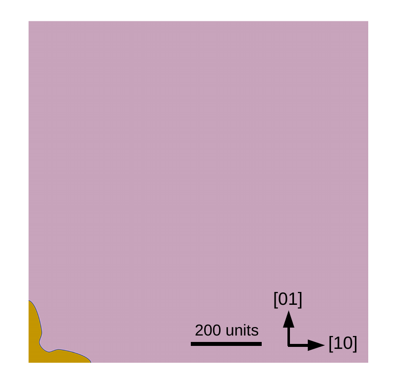
This section presents the specific details for the solidification and dendritic growth benchmark problem, including the model parameterization, initial conditions, boundary conditions, and computational domain size. The model is parameterized with dimensionless units, see the table below. While the diffuse interface width depends on orientation, it varies between four and five units, where the width is defined as the distance over which $-0.9 < \phi < 0.9$. The benchmark problem is formulated for two dimensions. To further reduce computational cost, we simulate one-quarter of a growing dendrite, as is commonly done in earlier works (e.g., Ref. [1, 2]). One-quarter of a solid seed with a radius of eight units (with the position of the interface defined as $\phi=0$) and a diffuse interface width of one unit is placed in the lower-left corner of the computational domain, surrounded by liquid. Initially, the entire system is uniformly undercooled with $U \left(t=0\right)=\Delta$. This undercooling is chosen to challenge numerical solvers somewhat because it increases the thermal diffusion length and requires a larger computational domain size relative to more negative undercoolings. We select a square computational domain of $(960 \textrm{ units})^2$, which is two times longer than the long dimension used in Ref. [1] for the same model parameterization. No-flux boundary conditions are chosen for $\phi$ and $U$ on all domain boundaries.
| Quantity | Symbol | Value |
|---|---|---|
| Interface thickness | $W_0$ | 1 |
| Rotational symmetry order | $m$ | 4 |
| Anisotropy strength | $\epsilon_4$ | 0.05 |
| Offset angle | $\theta_0$ | 0 |
| Relaxation time | $\tau_0$ | 1 |
| Diffusion coefficient | $D$ | 10 |
| Undercooling | $\Delta$ | -0.3 |
Example Result at $t=1500$
Submission Guidelines
All solutions should be run to at least $t=1500$. The following data should be collected for upload as frequently as possible.
The solid fraction in the domain (the integral of $\int_V \frac{\phi + 1}{2} dV$)
The free energy, $\mathcal{F}$
The estimated tip position versus time (the position of the $\phi=0.5$ contour line cutting either the $x=0$ or $y=0$ lines)
Three uploads are required for each data combination of time versus quantity. These should be named as free_energy, solid_fraction and tip_position and stored in either CSV or JSON format. The results can be stored in three separate files or one single file as long as each column name for time and quantity is identified on the upload form. In addition the phase field zero level set contour at time $t=1500$ is required. The data should be named as phase_field_1500 and include two columns for the x and y coordinates along the zero contour. The contour data should be in a sequence that enables an ordered traversal of the contour line.
Further data to upload can include a Youtube video, images of the dendrite at different times or the entire phase field variable at different times. These are not required, but will help others view your work.
Please use the upload form to upload your results.
Results
Results from this benchmark problem are displayed on the simulation result page for different codes.