Demos

Finding a Lorentzian peak

Files:

• demos/find_peak/sequentialLorentzian.py

Features:

• OptBayesExpt configuration and usage.

• Known measurement noise

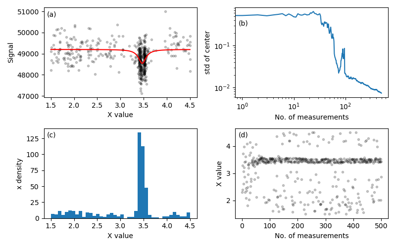
Figure 1. Plots generated by demos/find_peak/sequentialLorentzian.py illustrating a sequential Bayesian experimental design approach to measurement of a Lorentzian peak. The unknown parameters are the peak position and amplitude and the background level, and the peak width is fixed. Panel (a) shows the true curve in red and the simulated measurement data after 500 measurements. The signal to noise ratio is approximately 1.0. The algorithm focuses measurement resources near the peak as quantified by the histogram in (c). Measurements far from the peak reduce uncertainty in the background level. Panels (b) and (d) illustrate how the process evolves. (b) plots the standard deviation of the peak center, and (d) plots the measurement settings. For the first 50-ish measurements, the settings are scattered and the standard deviation drops slowly. After 50-ish measurements, the standard deviation drops quickly and the settings concentrate on the peak level. At around 150 measurements, the system enters a steady-state pattern of settings near the peak with less frequent measurements of the background. In this stage, the standard deviation typically reduces proportional to \(1/\sqrt{N}\).

---

Files:

• demos/find_peak/seqLor_pdfevolve.py

Features:

• OptBayesExpt configuration and usage.

• Animation of the data collection and of the parameter distribution.

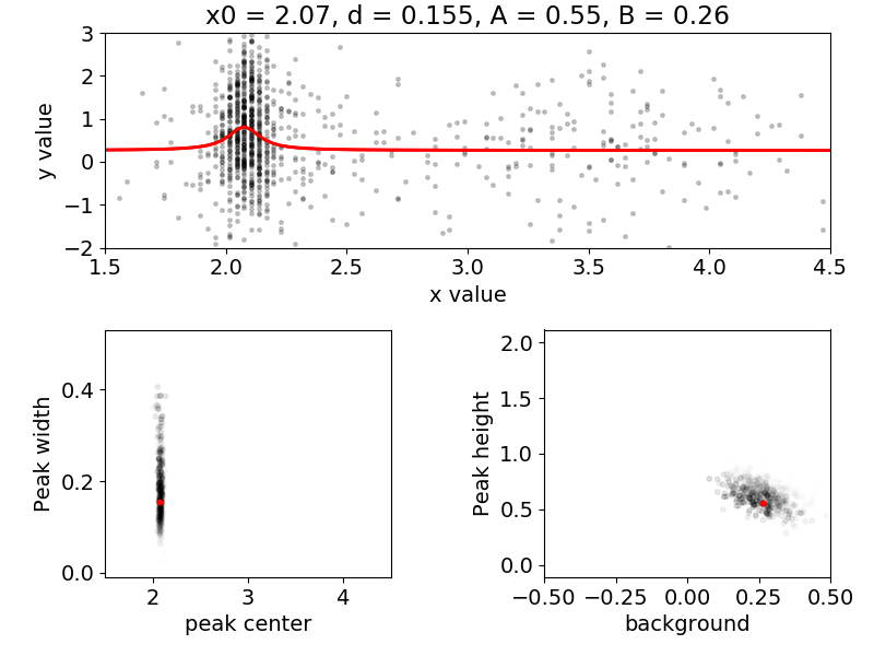
Figure 2. A snapshot of demos/find_peak/seqLor_pdfevolve.py. This program animates the evolution of the probability distribution function as simulated measurement results are incorporated. Four parameters are determined: the peak center x0, the peak width d, the peak amplitude A and the baseline value B. The top panel shows the true curve in red and the simulated data. The bottom two panels show 2D views of the 4D parameter space. As measurement data is incorporated, samples from the parameter distribution congregate around the true values, which are plotted as red dots.

Measurement speedup

Files:

• demos/fit_vs_obe_makedata.py

• demos/fit_vs_obe_plots.py

Features:

• OptBayesExpt configuration and usage.

• Known measurement noise

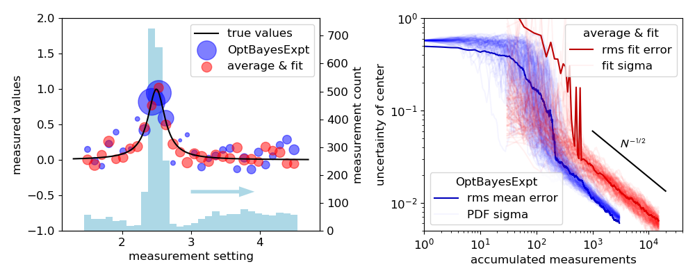
Figure 3: A different view of the Lorentzian peak problem, contrasting efficiency differences between experiment designs. The left panel shows results after 3000 measurements of a spectrum simulated with demos/fit_vs_obe_makedata.py and plotted with demos/fit_vs_obe_plots.py. The simulated experimental noise is Gaussian with standard deviation \(\sigma = 1\). In the “average & fit” method, 100 simulated measurements are averaged at each of 30 points, yielding a uniform uncertainty of \(\sigma_y = 1/\sqrt{100}\). In the OptBayesExpt method, the algorithm focuses attention on the sides of the peak, as shown in the histogram. The symbol areas are proportional to the weights of the data points, \(1/\sigma^2\). The smallest points correspond to \(\sigma_y = 0.258\), and the largest to \(\sigma_y \approx 0.037.\)

The right panel compares the evolution of runs using OptBayesExpt and average & fit runs. Faint lines trace the progress of 100 runs, each with 3000 OptBayesExpt measurements and 15 000 average & fit measurements. Faint lines trace the progress of uncertainty in \(x_0\) vs. the number of accumulated measurements: standard deviation of the \(x_0\) distribution for OptBayesExpt and standard deviation of the fit for the average & fit design. Dark lines plot the root-mean-square difference between the true values and either \(x_0\) distribution mean values or the best-fit values. Both the average & fit technique and the OptBayesExpt method scale like \(\sigma_{x0} \propto 1/\sqrt{N}\) (\(N\) = measurement number) for large \(N\), but the OptBayesExpt requires approximately 4 times fewer measurements to achieve the same uncertainty.

Details: The average & fit method used scipy.optimize.curve_fit(). The uncertainty plotted here is the square root of the diagonal element in the covariance matrix. For both methods, the peak height, background level and peak center are treated as unknowns, and the half-width line width is fixed at 0.3.

External experiment control

Files:

• demos/instrument_controller.py

• demos/server_script.py

Features:

• Simulated measurements and Bayesian experiment design run in separate processes.

• OBE_Server configuration an usage

This demo simulates a user’s instrumentation control program that communicates with an external OptBayesExpt class. The goal is to allow existing instrumentation software written in the user’s favorite language (UFL) to use the optbayesexpt package with python script and a little bit of UFL programming.

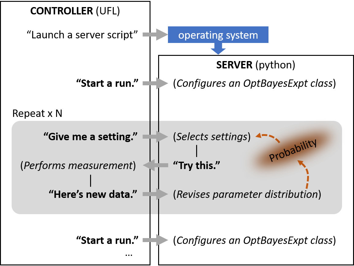
Figure 4. In this example, the instrument_controller.py program first launches the server_script.py script, which then runs “in the background” in a separate process. Then, the controller performs three measurement runs, each with a differently configured OptBayesExpt object. The flowchart of one such run is shown in the figure.

Tuning a pi pulse

Files:

• demos/pipulse/pipulse.py

Features:

• Multiple setting “knobs”

• Parameter distribution evolution

• Known measurement noise

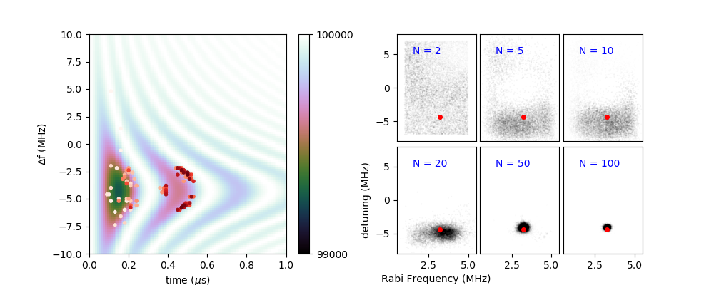
Figure 5: This demo, demos/pipulse/pipulse.py features a simulated measurement with more than one control setting. Radio frequency pulses can be used to manipulate spins, but in order to be accurate, both the duration and frequency of the radio-frequency pulse must be tuned. On the left, the background image displays the model photon counts for optically detected spin manipulation for different pulse durations (x-axis) and amounts of detuning from the spin’s natural resonance frequency (y-axis). In the background image, white indicates the expected measurement result for spin up and black, spin down. Points indicate simulated measurement settings, with sequence in order from white to dark red. Simulated measurements have 1\(\sigma\) uncertainties of \(\sqrt{N} \approx 316\). The right panel displays the evolution of the probability distribution function with the number “N” of measurements.

Slope Intercept

Files:

• demos/line_plus_noise/line_plus_noise.py

• demos/line_plus_noise/obe_noiseparam.py

Features:

• Comparison of setting selection methods

• Unknown measurement noise

• Customizing OptBayesExpt using a child class

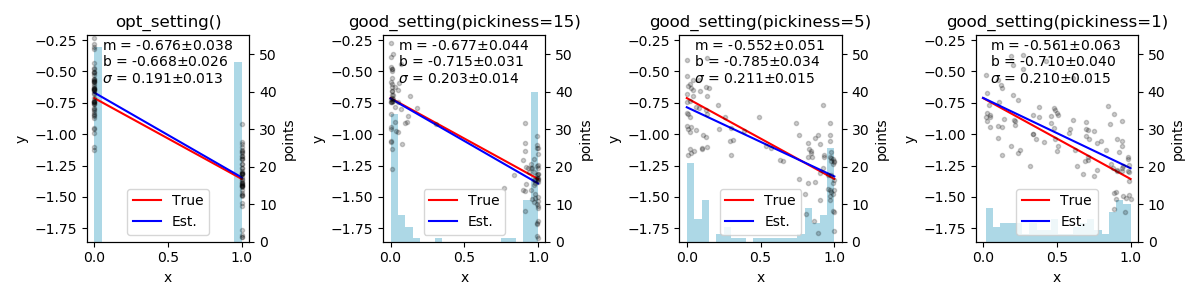
Figure 6: This demo demos/line_plus_noise/line_plus_noise.py, highlights the difference between algorithms for measurement selection opt_setting() method used in the first panel selects the setting with the highest utility \(\max[U(x)]\). As expected for a linear model, points at the ends of x’s range are most effective. The other three panels use the more flexible good_setting() method, selecting settings with a probability based on the utility and the pickiness parameter. The 2nd through 4th panels show that the good_setting() algorithm selects more diverse setting values as the pickiness is reduced. Note also that the standard deviations increase from left to right as measurement resources are diverted away from reducing uncertainty. Each run uses 100 points. See demos/line_plus_noise.py.

Additionally, this demo treats the measurement uncertainty as an unknown. The OptBayesExptNoiseParameter class provided in demos/line_plus_noise/obe_noiseparam.py inherits from OptBayesExpt. An added attribute, OptBayesExptNoiseParameter.noise_parameter_index identifies the noise parameter among the model parameters. The child class also adapts the likelihood() and yvar_noise_model() methods to handle distributions of the measurement uncertainty parameter.

A Lockin Amplifier

Files:

• demos/lockin/lockin_of_coil.py

Features:

• Multiple measurement inputs

• Setting-dependent measurement cost

• Unknown measurement noise

• Customizing OptBayesExpt using a child class

• trace_sort() utility

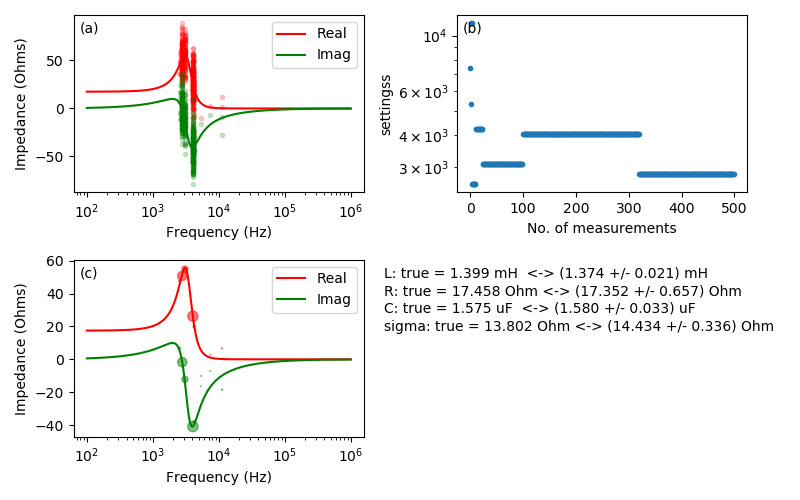
Figure 7. This demo simulates lockin measurement of a coil of wire. The circuit model consists of an inductance L in series with resistance R, and also a capacitance C in parallel with L and R to represent turn-to-turn capacitance. The lone setting is the measurement frequency and the instrument outputs are the X and Y channels, corresponding to the real and imaginary parts of the coil’s complex impedance. Panel (a) shows the “true” frequency response of the coil with raw data plotted.

Panel (b) shows the effects of a setting-dependent cost model on the setting choices. In the cost model used here, the cost of repeating a measurement is 1 time constant, and the cost of changing settings is assumed to be 5 time constants: 4 for settling time plus 1 for the measurement. The effect of adding a time cost for changing settings is that the settings exhibit a “sticky” behavior. After a few short measurements, settings tend to be chosen in long periods of repeated measurements with infrequent setting changes. Please note that this cost model is just a sketch for demonstration purposes. It may not be suitable for any actual measurements.

Panel (c) demonstrates the use of the optbayesexpt.trace_sort() utility function. The trace_sort() function sorts the raw data and computes the mean and standard deviation of mean, \(\sigma\) at each setting. Symbol areas are proportional to the statistical weight = \(1/\sigma^2\) of the mean.

Opinion:

The aesthetic problem that trace_sort() addresses can be seen in panel (a) and in similar plots of raw data. While these plots are honest representations, the visual impact of large collections of markers disagrees with the fact that many points produce the most precisely known mean values. After computing mean values and standard deviations, \(\sigma\), the next step traditionally would be an error bar plot, but the error bars have a similar visual problem: the most important points on the plot have small error bars and low visual impact, while less important plots have big, eye-catching error bars. By plotting mean values with symbol areas proportional so statistical weight, the visual impact of the data is in harmony with its importance.

A Sweeper

Files:

• demos/sweeper/sweeper.py

• demos/sweeper/obe_sweeper.py

Features:

• Swept-setting measurements

• Separation of measurement-point settings from sweep property controls

• Many data points per measurement

• Unknown measurement noise

• Setting-dependent cost

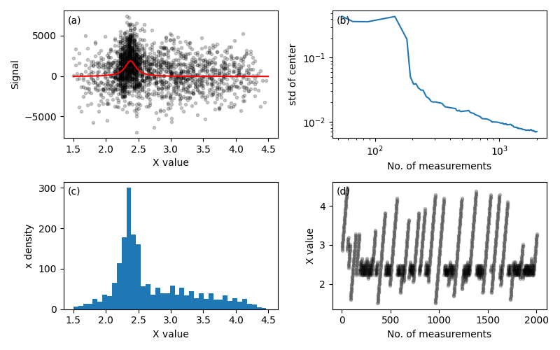
Figure 8. This demo takes on the challenge of a spectrometer-like instrument that accepts sweep limits as controls and returns data as arrays of settings and corresponding results. The model function is the tried-and-true Lorentzian peak with the peak center, amplitude, background, and noise \(\sigma\) as unknown parameters and with constant peak width. The cost function includes a constant value for the cost of a new sweep plus a term corresponding to the length of the sweep. In this simulation, the setup cost is the same as the cost of 5 data points.

Panel (a) shows the true curve in red with the simulated measurement data, which is concentrated around the peak position as shown by the histogram in (c). Panel (b) shows the standard deviation of the peak center distribution vs. the number of accumulated data points. The standard deviation begins to drop dramatically after about 300 or 400 measurements. Panel (d) traces the measurement settings. The strategy that emerges typically begins with a broad sweep followed by shorter sweeps focused on possible peak positions. Later in the process, the algorithm includes an occasional broad sweep, presumably to decrease uncertainty in the baseline parameter.

Code speedup with numba

Files:

• demos/numba/numbaLorentzian.py

• numba python package required

Features:

• Improved execution time using pre-compilation.

This numbaLorentzian.py script demonstrates the use of numba and its @njit decorator to accelerate the more numerics-intensive functions in optbayesexpt. The purpose of numba is to pre-compile Python code just-in-time (jit) so that when the function is called, the CPU runs machine code without involvement from the Python interpreter.

In numbaLorentzian.py, the Boolean variable use_jit enables (use_jit = True) or disables ( use_jit = False) pre-compilation. In this demo, we use numba to pre-compile three of the more numerically demanding functions in optbayesexpt.

• _gauss_noise_likelihood() – the calculation of likelihood

• my_model_function() – the guts of the experiment model calculation

• _normalized_product() – Bayes’ rule multiplication of likelihood and prior with normalization.

The output of numbaLorentzian.py includes a code profile that shows where the computation time was spent. Table I below compares execution times of the most time consuming functions without (use_jit = False) and with (use_jit = True) pre-compilation. The times listed represent time spent on a function, not counting called functions. Pre-compilation roughly halved the execution time of the most time-consuming function, which calculates a Gaussian likelihood. The most dramatic improvement is in calculation of the model function which was sped up by nearly a factor of five.

Table I.

uses jit
False	True
time (s)	time (s)	filename:lineno(function)
4.150	2.000	obe_base.py:199(_gauss_noise_likelihood)
2.724	0.538	numbaLorentzian.py:101(my_model_function)
2.259	1.747	{method ‘choice’ of ‘numpy.random._generator.Generator’ objects}
0.850	0.827	particlepdf.py:129(_normalized_product)
…	…	…
13.109 s	8.322 s	Total

The overall execution time is shown in the last line of Table I. With numba pre-compilation, there is a significant, but not spectacular decrease in execution time.

Speculation:

Compared to examples in the numba documentation (see https://numba.pydata.org/numba-doc/latest/user/5minguide.html#how-to-measure-the-performance-of-numba) the acceleration in this example seems small. One possible explanation for the small speed increase is that much of the computation already takes advantage of math using numpy arrays, which are pre-compiled operations.