Example linear regression (2nd-order polynomial)
This is a toy problem meant to demonstrate how one would use the ML Uncertainty toolbox. The problem being solved is a linear regression problem and has an uncertainty that can already be calculated analytically.
Imports
[1]:
%matplotlib inline
import scipy as sp
import matplotlib.pyplot as plt
import numpy as np
import sklearn.linear_model as sklm
import sklearn.model_selection as skcv
import ml_uncertainty as plu
Data and Metadata
Data for the toy problem
Here’s some X data
[2]:
xdata = np.array([[4.00],
[4.20],
[4.30],
[4.47],
[4.58],
[4.60],
[4.61],
[4.82],
[5.05],
[5.24],
[5.43],
[5.58],
[5.82],
[5.91],
[5.92],
[6.03],
[6.32],
[6.45],
[6.67],
[6.68],
[6.91],
[7.04],
[7.09],
[7.35],
[7.49],
[7.62],
[7.81],
[7.94]])

#Create the linear regression X matrix
xmatrix_first = np.ones_like(xdata) #Constant term
xmatrix_last = xdata**2 #Square term
#Add in the linear term
xmatrix = np.concatenate((xmatrix_first,xdata,xmatrix_last),axis=1)
Here’s some Y data
[3]:
yfull = np.array([[3.70,3.53,4.12,5.03,],
[2.96,4.69,6.44,7.36,],
[4.69,3.68,5.86,5.70,],
[4.28,4.22,5.32,6.33,],
[4.86,5.27,5.61,5.57,],
[4.77,4.61,5.38,4.91,],
[4.74,4.45,6.34,5.71,],
[4.76,4.40,6.51,5.62,],
[5.01,5.52,5.85,6.92,],
[5.59,5.81,5.86,7.98,],
[5.17,4.67,5.58,8.38,],
[6.02,6.04,5.70,6.87,],
[6.68,5.94,5.78,8.10,],
[6.91,5.97,5.68,7.80,],
[6.14,5.74,6.30,7.65,],
[5.67,5.78,4.97,8.98,],
[6.89,6.41,6.40,8.08,],
[6.57,6.46,6.44,8.43,],
[7.34,6.31,6.14,8.55,],
[6.62,5.98,5.78,9.17,],
[7.22,6.59,5.99,8.95,],
[8.05,6.85,6.78,10.92,],
[7.11,7.29,6.19,9.74,],
[6.43,7.40,6.45,9.39,],
[7.02,7.14,7.34,10.13,],
[7.27,7.37,6.12,10.04,],
[7.29,7.07,5.65,10.91,],
[8.29,8.39,6.57,11.78,]])

ydata = yfull[:,0]

#Make the data into a 2nd-order monomial with 2x the residual
# of the linear data
resid = ydata-np.squeeze(xdata)
ysquared = np.squeeze(xdata**2) + 2*resid
Sklearn models
Make some sklearn models that we’ll use for regression.
[4]:
linear_regressor = sklm.LinearRegression
regr = linear_regressor()
cv = skcv.KFold(n_splits=6,shuffle=True)
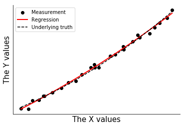
Regression
Recall the generic for for the linear regression problem and the way to calculate the coefficients. Here, Y is the array of dependent variable measurements and X is the array of independent variable measurements. To account for the constant term, X must be prepended by a column consisting of all ones.
[5]:
regr.fit(xmatrix[:,1:],ysquared)
ypred = regr.predict(xmatrix[:,1:])
y_cv = skcv.cross_val_predict(regr,xmatrix[:,1:],y=ysquared,cv=cv)
[7]:
#with plt.xkcd():
fig,ax = plt.subplots(1,1)

p1 = plt.scatter(xdata,ysquared,color='k',label='Measurement')
p2 = plt.plot(xdata,ypred,color='r',lw=2,label='Regression')
p3 = plt.plot(xdata,xdata**2,color='k',ls='--',label='Underlying truth')

handles, labels = ax.get_legend_handles_labels()

plt.legend([handles[i] for i in [2,0,1]],[labels[i] for i in [2,0,1]])
ax.set_xlabel('The X values',size=15)
ax.set_ylabel('The Y values',size=15)
ax.set_xticks([])
ax.set_yticks([])
ax.spines['right'].set_visible(False)
ax.spines['top'].set_visible(False)
ax.set_ylabel

t = 1
Uncertainty Calculation
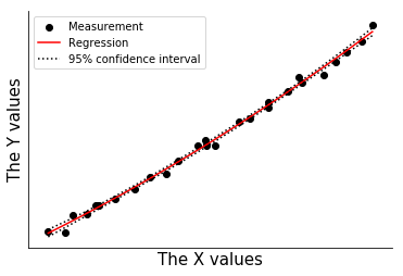
Traditional uncertainty calculation
This is the equation for the 95% confidence interval for a new prediction \(X_{new}\) (in linear regression).
Here, \(t\) is the 95th percentile of the one-sided Student’s T distribution with \(n\) - 2 degrees of freedom, with \(n\) being the number of samples in the regression (i.e. number of rows of \(X\)).
Calculate the values for the \(t\) distribution and the SSE term.
[25]:
#Create the linear regression X matrix
#xmatrix_first = np.ones_like(xdata) #Constant term
#xmatrix = np.concatenate((xmatrix_first,xdata),axis=1) #Add in the linear term

cov = np.dot(xmatrix.T,xmatrix) #Covariance matrix
icov = np.linalg.inv(cov) #Inverse covariance matrix
xty = np.dot(xmatrix.T,ysquared[:,np.newaxis,]) #XTy

beta = np.dot(icov,xty) #Coefficients

nvars = xmatrix.shape[1]
nsamp = xmatrix.shape[0]

dof = nsamp - nvars#Degrees of freedom
tdist = sp.stats.t(dof) #T distribution
#T premultiplier, only one standard deviation because n is large. Squared because of how pred_unc is defined below
tmult = tdist.ppf(0.95) ** 2

sse = (np.dot(ysquared.T,ysquared) - np.dot(ypred.T,ysquared))/(dof) #mean squared error

var_premult = tmult * sse
Calculate the uncertainty in the predicted values
[11]:
yl = []
yu = []
for row in xmatrix:

    yp = np.dot(row,beta)
    pred_unc = np.sqrt(var_premult*(np.dot(np.dot(row,icov),row.T)))

    yl += [yp - 1*pred_unc]
    yu += [yp + 1*pred_unc]

    #print(pred)

    #print(pred,pred_lower,pred_upper)
lower = np.concatenate(yl)
upper = np.concatenate(yu)

yunc = np.concatenate((yl,yu),axis=1)

fig,ax = plt.subplots()

ax.plot(xdata,ypred,color='r',label='Regression')
ax.plot(xdata,yunc,ls=':',color='k',label='95% confidence interval')
ax.scatter(xdata,ysquared,color='k',label='Measurement')

handles, labels = ax.get_legend_handles_labels()

ax.legend([handles[i] for i in [3,0,1]],[labels[i] for i in [3,0,1]])

ax.set_xlabel('The X values',size=15)
ax.set_ylabel('The Y values',size=15)
ax.set_xticks([])
ax.set_yticks([])
ax.spines['right'].set_visible(False)
ax.spines['top'].set_visible(False)
#plt.legend()
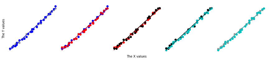
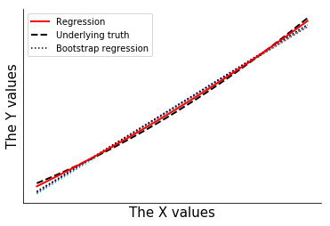
Bootstrap uncertainty calculation
Use the residual bootstrap of Almeida This method assumes that the residuals are representative of the uncertainty (which is really the same assumption made by linear regression uncertainty, when you think about it).
Calculate the mean squared error and the cross-validation error in the regression, then calculate the pseudo-degrees of freedom and the residual weighting that will be bootstrapped. This is a large data set and cross-validation doesnt give us much more information, so the bootstrap weighting is close to 1.
[12]:
residual,err,mse = plu.get_residual_stats(ysquared,ypred)
residual_cv,err_cv,msecv = plu.get_residual_stats(ysquared,y_cv)

num_train = len(xdata)

pseudo_dof = num_train * (1 - np.sqrt(mse/msecv))
bootstrap_weight = np.sqrt(1 - pseudo_dof/num_train)

print(bootstrap_weight)

residual_weighted = residual / bootstrap_weight
0.9406480574386638
[13]:
samples = 5

residual_boot,boot_indices = plu.bootstrap_data(residual_weighted,samples=samples)
residual_boot = np.squeeze(residual_boot)

boot_data = (residual_boot + ypred).T #boot_data now has the new Y values with shuffled residuals
Create some plots, generate and plot five regressions.
[14]:
fig,axes = plt.subplots(1,samples,figsize=(3*samples,3),sharey=True,
                        gridspec_kw=dict(wspace=0),subplot_kw=dict(frameon=False))
fig2,ax2=plt.subplots(1,1)

colors = '0.6','b','r','k','c'
ax2.plot(xdata,ypred,color='r',lw=2,zorder=100,label='Regression')
ax2.plot(xdata,xdata**2,color='k',ls='--',lw=2,zorder=99,label='Underlying truth')

ax2.set_xticks([])
ax2.set_yticks([])

ax2.set_xlabel('The X values',size=15)
ax2.set_ylabel('The Y values',size=15)

ax2.spines['right'].set_visible(False)
ax2.spines['top'].set_visible(False)

for ax in axes:
    ax.spines['right'].set_visible(False)
    ax.spines['left'].set_visible(False)
    ax.spines['top'].set_visible(False)
axes[0].spines['left'].set_visible(True)

for plot_num,(color,yboot) in enumerate(zip(colors,boot_data.T)):

    yb = yboot[:,np.newaxis]

    #fig,ax = plt.subplots(1,1)
    regr.fit(xdata,yb)
    ypb = regr.predict(xdata)

    #print('{},{}'.format(plot_num-1,plot_num+1))

    for ax in axes[[plot_num-1,plot_num]]:
        ax.scatter(xdata,yb,color=color)
        ax.plot(xdata,ypb,color=color)
        ax.set_xticks([])
    if color=='k':
        ax2.plot(xdata,ypb,color=color,ls=':',label='Bootstrap regression')
    else:
        ax2.plot(xdata,ypb,color=color,ls=':')

ax = axes[0]
ax.set_yticks([])
ax.set_ylabel('The Y values')
ax = axes[2]
ax.set_xlabel('The X values')


ax2.legend()
[14]:
<matplotlib.legend.Legend at 0x7ff54fed1978>
Using the toolbox
Now do the same thing with 1000 samples. This time we’ll just use the bootstrap() function, and we can just drop the data straight in.
[15]:
samples = 1000

linear_bootstrap = plu.bootstrap_estimator(estimator=linear_regressor,
                                           X=xmatrix[:,1:],y=ysquared,samples=samples,cv=cv,
                                          )

linear_bootstrap.fit()

ypred,cpb,bounds,error, = linear_bootstrap.bootstrap_uncertainty_bounds()

#lbt_out = plu.bootstrap(xdata=xdata,ydata=np.squeeze(ydata),
#                        PLS_model=regr,cv_object=cv,samples=samples)
#rcv,ecv,msecv,cpb,cpt = lbt_out
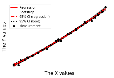
Plot the bootstrap results and show that the bootstrap uncertainty exactly reproduces the results of the linear regression uncertainty.
[16]:
fig2,ax2=plt.subplots(1,1)

for ypb in cpb:
    ax2.plot(xdata,ypb,color='0.6',ls=':',zorder=0)

ax2.plot(xdata,ypred,color='r',lw=3,label='Regression',zorder=3)
ax2.plot(xdata,yunc,ls='--',color='r',lw=3,label='95% CI (regression)',zorder=3)
ax2.plot(xdata,ypb,color='0.6',ls=':',label='Bootstrap',zorder=-1)

ax2.plot(xdata,bounds.T,ls=':',color='k',lw=3,label='95% CI (boot)',zorder=4)

ax2.scatter(xdata,ysquared,color='k',label='Measurement',zorder=5)

ax2.set_xlabel('The X values',size=15)
ax2.set_ylabel('The Y values',size=15)

ax2.set_xticks([])
ax2.set_yticks([])


ax2.spines['right'].set_visible(False)
ax2.spines['top'].set_visible(False)

#ax2.legend()

handles, labels = ax2.get_legend_handles_labels()

ax2.legend([handles[i] for i in [0,3,1,4,6]],[labels[i] for i in [0,3,1,4,6]])

t = 1
[17]:
(yunc - bounds.T)/error.T
[17]:
array([[ 0.09483087, -0.10595275],
       [ 0.10746581, -0.10633848],
       [ 0.10166273, -0.12672244],
       [ 0.08929502, -0.11990567],
       [ 0.12438105, -0.09780311],
       [ 0.1261887 , -0.09332473],
       [ 0.12626065, -0.0912731 ],
       [ 0.10391902, -0.10553357],
       [ 0.12381275, -0.14610142],
       [ 0.1451628 , -0.12070537],
       [ 0.16982132, -0.10073642],
       [ 0.18724042, -0.07826695],
       [ 0.19304763, -0.10100713],
       [ 0.16893004, -0.07911934],
       [ 0.16634934, -0.07878156],
       [ 0.14194964, -0.07905529],
       [ 0.16571014, -0.10854832],
       [ 0.16550811, -0.10531119],
       [ 0.15156991, -0.12251177],
       [ 0.14921162, -0.12882945],
       [ 0.16454438, -0.18028952],
       [ 0.16855882, -0.1692009 ],
       [ 0.15441342, -0.17368161],
       [ 0.13762857, -0.14694859],
       [ 0.12559564, -0.1587315 ],
       [ 0.10218068, -0.17468748],
       [ 0.11006489, -0.17726765],
       [ 0.11500796, -0.18186523]])
[18]:
yunc
[18]:
array([[14.27109377, 15.97394449],
       [16.37680081, 17.76217485],
       [17.43537962, 18.686175  ],
       [19.24163371, 20.30478879],
       [20.41382092, 21.38525244],
       [20.62718987, 21.58454258],
       [20.73390178, 21.68451633],
       [22.97968771, 23.83396889],
       [25.45728854, 26.29032594],
       [27.53107877, 28.38713721],
       [29.64108567, 30.5334338 ],
       [31.33772939, 32.25756711],
       [34.11528272, 35.06436097],
       [35.17772189, 36.13130615],
       [35.29648349, 36.25032982],
       [36.61228694, 37.56583283],
       [40.16305744, 41.08983596],
       [41.79175482, 42.69739948],
       [44.59475653, 45.46254661],
       [44.72342105, 45.58970988],
       [47.70695501, 48.55573803],
       [49.40911429, 50.27192671],
       [50.06582826, 50.94064503],
       [53.49222197, 54.50217208],
       [55.34336183, 56.48023124],
       [57.06665282, 58.35428906],
       [59.59531748, 61.15545813],
       [61.33396394, 63.11291955]])
[19]:
bounds.T
[19]:
array([[14.18157366, 16.07448446],
       [16.29375706, 17.84495417],
       [17.36485319, 18.77724574],
       [19.18972835, 20.37751209],
       [20.345278  , 21.43825215],
       [20.55910007, 21.63455203],
       [20.66618914, 21.73293219],
       [22.930696  , 23.88491853],
       [25.39865577, 26.36186427],
       [27.45871042, 28.44615106],
       [29.54993178, 30.5834779 ],
       [31.23250963, 32.29689087],
       [34.00278657, 35.11816107],
       [35.08238569, 36.17293874],
       [35.20275709, 36.29173306],
       [36.53421263, 37.60717462],
       [40.07044362, 41.14590933],
       [41.70143859, 42.75039947],
       [44.51842314, 45.52404836],
       [44.64837753, 45.65454068],
       [47.62405831, 48.64984816],
       [49.32231381, 50.36044898],
       [49.98640955, 51.03310856],
       [53.41225758, 54.58983612],
       [55.26336696, 56.58965504],
       [56.99503156, 58.49363263],
       [59.50055003, 61.32651216],
       [61.2181546 , 63.31027015]])
[20]:
error.T
[20]:
array([[0.94399751, 0.94891328],
       [0.77274589, 0.77845123],
       [0.69372945, 0.7186631 ],
       [0.58127947, 0.60650427],
       [0.551072  , 0.54190215],
       [0.53958709, 0.53586486],
       [0.53629251, 0.53045055],
       [0.47144125, 0.48278128],
       [0.47356007, 0.48964844],
       [0.49853236, 0.48890829],
       [0.53676354, 0.49678258],
       [0.56195001, 0.50243122],
       [0.58273782, 0.53263669],
       [0.56435315, 0.52619991],
       [0.56343114, 0.52554483],
       [0.55001416, 0.52294783],
       [0.55889049, 0.51657522],
       [0.54569065, 0.50327023],
       [0.50361838, 0.50200684],
       [0.50293351, 0.50322964],
       [0.50379542, 0.52199443],
       [0.51495664, 0.52317854],
       [0.51432522, 0.53237379],
       [0.58101593, 0.59656261],
       [0.63692399, 0.6893641 ],
       [0.70092757, 0.7976735 ],
       [0.86101429, 0.96494784],
       [1.00696801, 1.08514754]])
[21]:
linear_bootstrap.boot_data.shape
[21]:
(1000, 28)
[22]:
linear_bootstrap.boot_data.std(axis=0)
[22]:
array([0.98414377, 0.9800988 , 0.96281945, 0.97785665, 0.99255599,
       0.96224198, 0.97777613, 0.9784806 , 0.97131318, 0.99204086,
       0.99410038, 0.95844077, 0.99162786, 0.95797863, 0.97178914,
       0.95407061, 0.97049178, 0.97078983, 0.99070464, 0.96782657,
       0.98975311, 0.96187947, 0.96709553, 0.94918955, 0.96550174,
       1.00714298, 1.00930739, 1.0094565 ])
[23]:
linear_bootstrap.base_predict(xmatrix[:,1:]).shape
[23]:
(28,)
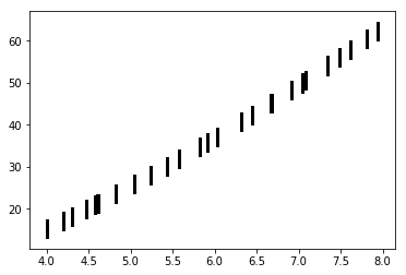
[24]:
ymodel = linear_bootstrap.base_predict(xmatrix[:,1:])
for row in linear_bootstrap.boot_data:
    plt.scatter(xdata,row+ymodel,s=1,color='k')
[ ]: