[14]:
%matplotlib inline
import matplotlib.pyplot as plt
from masskit.data_specs.spectral_library import LibraryAccessor
Read and analyze predicted spectra
[15]:
df = LibraryAccessor.read_sql('/aiomics/results/DB210814_HmAll.db')
Display first 10 rows
[16]:
df[:20][['spectrum', 'predicted_spectrum', 'cosine_score', 'nce', 'charge', 'peptide']].lib.display()
| spectrum | predicted_spectrum | cosine_score | nce | charge | peptide |
|---|---|---|---|---|---|
 |
 |
679.90 | 35.00 | 2 | AAAACALTPGPLADLAAR |
 |
 |
645.16 | 35.00 | 2 | AAAACALTPGPLADLAAR |
 |
 |
259.16 | 35.00 | 3 | AAAALGSHGSCSSEVEKETQEK |
 |
 |
689.39 | 34.00 | 3 | AAAALGSHGSCSSEVEKETQEK |
 |
 |
558.94 | 35.00 | 3 | AAAALGSHGSCSSEVEKETQEK |
 |
 |
466.45 | 35.00 | 4 | AAAALGSHGSCSSEVEKETQEK |
 |
 |
615.67 | 35.00 | 2 | AAAASAAEAGIATSGTEGER |
 |
 |
681.65 | 35.00 | 2 | AAAASGEPLHNEEER |
 |
 |
643.82 | 34.00 | 3 | AAAASGEPLHNEEER |
 |
 |
769.23 | 34.00 | 2 | AAADLGTEAGVQQLLCTVR |
 |
 |
648.41 | 35.00 | 2 | AAAPSSPSSPAEMQSLK |
 |
 |
660.45 | 34.00 | 2 | AAAPSSPSSPAEMQSLK |
 |
 |
697.16 | 34.00 | 2 | AAATEDATPETLEK |
 |
 |
759.23 | 34.00 | 2 | AAATEENVTWR |
 |
 |
637.99 | 35.00 | 2 | AAATEENVTWR |
 |
 |
773.97 | 35.00 | 2 | AAAVSDIQELMR |
 |
 |
750.27 | 34.00 | 2 | AAAVSDIQELMR |
 |
 |
710.36 | 35.00 | 2 | AAAVSDIQELMR |
 |
 |
678.46 | 34.00 | 2 | AAAVSDIQELMR |
 |
 |
671.95 | 34.00 | 2 | AACADDFIGEMPDGIHTEIGEK |
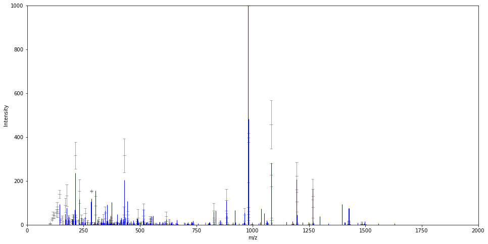
Plot two spectra, one with error bars
[17]:
fig, ax = plt.subplots(figsize=(16, 8))
# select spectra from the 2nd row of the datafram
experimental_spectrum = df.iloc[1]['spectrum']
predicted_spectrum = df.iloc[1]['predicted_spectrum']
experimental_spectrum.plot(ax, predicted_spectrum, normalize=1000, mirror=False, plot_stddev=True)
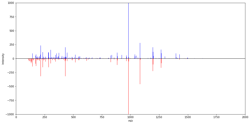
Plot two spectra with a mirror plot, no error bars
[18]:
fig, ax = plt.subplots(figsize=(16, 8))
experimental_spectrum.plot(ax, predicted_spectrum, normalize=1000, mirror=True)
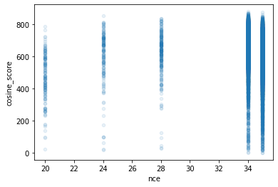
Plot relationship between cosine score and various spectrum properties
[19]:
df.plot.scatter('nce', 'cosine_score', alpha=0.1)
plt.show()
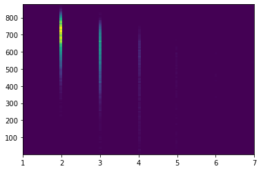
[20]:
plt.hist2d(df['charge'], df['cosine_score'], bins = 100)
plt.show()
[21]:
df['predicted_spectrum'].iloc[1]
[21]:

[22]:
df['spectrum'].iloc[1]
[22]:

Compute the cosine score, which automatically changes the mass tolerance of the experimental spectra to evenly spaced bins instead of ppm
[23]:
# get the experimental spectrum from the 5th row
experimental_spectrum = df['spectrum'].iloc[1]
# get the predicted spectrum from the 5th row
predicted_spectrum = df['predicted_spectrum'].iloc[1]

# convert the experimental spectra, which has ions in +/- 10ppm bins into a spectrum with evenly spaced bins
# that are the same size as the

df['predicted_spectrum'].iloc[1].cosine_score(df['spectrum'].iloc[1])
[23]:
645.1566559109622
Access mz, intensity, and std deviation of the intensity for an example spectrum
[24]:
print(df['predicted_spectrum'].iloc[1].products.mz)
print(df['predicted_spectrum'].iloc[1].products.intensity)
print(df['predicted_spectrum'].iloc[1].products.stddev)
[ 101.1  110.1  115.1  120.1  129.1  133.   136.1  143.1  147.1  155.1
  157.1  169.1  175.1  183.1  185.1  187.1  197.1  201.1  204.1  214.1
  215.1  226.1  232.1  240.1  246.2  252.1  257.2  268.2  282.2  283.1
  285.2  286.2  297.2  300.2  303.1  311.2  317.2  325.2  331.1  337.2
  345.2  346.2  354.2  365.2  374.1  374.2  382.2  388.2  396.2  400.2
  413.7  416.2  417.2  428.2  430.3  431.3  445.2  446.2  459.2  471.2
  473.2  487.2  488.2  490.8  491.3  499.2  516.2  517.2  518.2  523.3
  541.8  545.3  551.3  558.3  559.3  574.2  584.3  585.3  599.3  601.3
  602.3  615.3  616.3  617.3  629.3  630.3  645.3  664.3  664.4  695.3
  698.3  712.3  712.4  713.3  713.4  729.4  730.3  730.4  735.4  789.4
  792.4  806.4  806.5  807.4  809.5  826.5  827.5  828.5  855.4  855.5
  856.4  856.5  863.4  883.5  884.4  884.5  885.5  892.5  911.5  912.5
  913.5  962.5  963.5  964.5  980.5  980.6  981.5  981.6  982.6  996.6
  997.6 1063.6 1064.6 1065.6 1081.6 1082.6 1083.6 1084.6 1176.7 1177.7
 1194.7 1195.7 1196.7 1247.7 1248.7 1265.7 1266.7 1267.7 1408.7 1425.7
 1425.8 1426.7 1426.8 1427.8 1482.8 1483.8 1484.8 1496.8 1497.8]
[5.16083876e+00 2.58119793e+01 4.52980728e+01 4.29759789e+01
 5.40103442e+01 8.13785731e+01 5.28966064e+01 1.39404416e+02
 1.94305776e+01 3.15372798e+01 9.79780221e+00 8.89233004e+01
 1.33486944e+02 2.88384527e+01 1.43848513e+01 1.02618426e+01
 1.69114602e+01 1.51254930e+01 4.04518827e+01 3.15514394e+02
 3.49380767e+01 1.71735137e+01 1.52572861e+02 2.83180704e+01
 1.96575836e+01 3.72736184e+00 5.21105804e+01 1.21028500e+01
 1.75061029e+00 5.65349054e+00 1.53297129e+02 1.09461603e+01
 1.45028400e+00 1.77932451e+00 8.78354390e+01 1.56785562e+00
 2.56543522e+01 5.52565002e+00 3.43558228e+00 2.47159878e+01
 5.55190131e+01 3.46792622e+00 2.91550646e+00 1.40627217e+01
 2.10881570e+01 2.19645234e+00 1.23521979e+00 6.15356863e+00
 8.67259731e-01 8.65324799e+00 6.18079935e+00 8.75124709e+00
 1.80809911e+01 4.64485399e+01 3.15463796e+02 2.44595464e+01
 4.53512669e+01 1.23150229e+01 3.86595956e+00 5.09977396e+00
 1.83562874e+00 1.49544491e+01 5.43874447e+00 3.19624180e+01
 4.90814301e+00 6.31941160e+00 6.76924305e+01 1.27176159e+01
 1.55018534e+00 7.30450143e-01 1.83815703e+00 2.74100609e+01
 2.53466485e+01 4.27236724e+00 1.32345770e+00 1.32219908e+00
 1.14340531e+00 1.92775601e-01 9.86801351e-01 2.89245967e+00
 9.07937927e-01 3.06256998e+00 3.80689144e+01 4.03895209e+00
 1.68299584e+01 1.24196566e+00 9.27341272e-01 1.21006152e-01
 2.10869348e+00 2.33358063e-01 1.48374622e-01 1.74693785e+00
 3.29419582e-01 2.26506269e+00 2.51234561e-01 3.76007085e-01
 9.09070335e-01 3.49084339e+00 5.00036569e+00 1.26826062e-01
 1.31171597e-01 3.05587870e+00 4.46120451e-01 8.58604210e-01
 2.08424346e-01 6.46612116e+01 1.24078199e+01 1.46774153e-01
 1.10346828e+01 5.66449400e+00 6.42823370e-01 1.18834637e+00
 9.95144238e-01 1.12347687e+02 1.50887308e-01 3.17686586e+01
 5.94285420e-01 6.40690317e-01 2.57784754e-01 1.47392961e+00
 1.74349088e-01 3.45054537e+00 4.61012249e+01 2.52312385e+00
 8.01442854e+01 9.98999980e+02 8.10851006e+00 3.96393392e+02
 4.76559747e+01 8.19021103e-01 1.26030604e-01 5.78518947e+00
 3.74937332e+00 1.42000185e-01 4.56191864e+02 2.26583435e+02
 2.04235824e+01 1.98942932e-01 2.04833768e+00 4.30711520e-01
 2.22584824e+02 1.04438843e+02 4.83105628e+00 5.98821977e-01
 3.32410534e-01 1.61986422e+02 8.05839043e+01 4.58331164e+00
 1.16798632e-01 4.68055431e+00 1.48945080e+01 1.59660129e+00
 1.00008792e+01 8.07077974e-01 1.50441566e+00 5.08685346e+00
 3.63960647e-01 1.07809912e+00 4.69608217e-01]
[1.16081091e+00 4.96569763e+00 1.48371552e+01 1.27593059e+01
 1.76112545e+01 2.11693998e+01 1.85390595e+01 1.82689739e+01
 7.35791736e+00 8.42747120e+00 6.91072252e+00 3.16643043e+01
 4.96361216e+01 1.43508389e+01 7.45341551e+00 7.39242769e+00
 8.35082195e+00 8.97107831e+00 7.07409758e+00 6.18156375e+01
 1.15464452e+01 3.71713669e+00 5.43287635e+01 1.71071001e+01
 5.82201529e+00 2.03797718e+00 2.36521319e+01 7.85772000e+00
 1.33865063e+00 4.21003791e+00 2.04501461e+00 7.58362664e-01
 1.13418525e-01 1.27134200e+00 4.15544046e+01 8.10988832e-01
 9.42590473e+00 3.90288281e+00 4.09635332e+00 2.26773672e+01
 2.57799952e+01 1.88067891e+00 3.15673693e+00 5.41396756e+00
 9.63515290e+00 1.20261899e+00 8.21626021e-01 5.24247016e+00
 7.53198709e-01 1.51155563e+00 7.08872063e+00 1.54069309e+00
 4.56097416e+00 3.57012778e+01 7.69583597e+01 9.48144697e+00
 1.57533782e+01 1.05827693e+01 2.40261904e+00 2.55019340e+00
 1.71943616e+00 9.69968681e+00 1.34746791e+00 3.89297543e+01
 6.93822100e+00 2.45914686e+00 2.76123852e+01 1.47921886e+01
 2.19150487e+00 5.97251048e-01 1.84109904e+00 1.22590466e+01
 6.91952208e+00 4.12884856e+00 1.68920695e+00 1.82976285e+00
 8.00143162e-01 2.17927403e-01 8.20364365e-01 2.54890460e+00
 1.06565540e+00 2.61824805e+00 2.14305536e+01 2.22171174e+00
 7.19407672e+00 7.27401970e-01 1.15247922e+00 6.75259005e-02
 6.73731607e-01 2.40965267e-01 1.09384899e-01 2.04967811e+00
 3.76881433e-01 2.44278738e+00 7.10590103e-02 4.82696090e-01
 6.85515683e-01 3.59404858e+00 3.26690169e+00 1.67276778e-01
 1.21202129e-01 2.78134761e+00 5.03134318e-01 9.94727104e-01
 1.30094650e-01 3.38483467e+01 1.03623444e+01 1.82474820e-01
 8.00854162e+00 5.71481867e+00 5.12452586e-01 1.19727587e+00
 9.29751544e-01 4.92026218e+01 1.18255071e-01 2.08285067e+01
 5.45585981e-01 7.02788423e-01 3.61643904e-01 2.07941376e+00
 2.43802000e-01 4.01163622e+00 2.86530775e+01 2.18161705e+00
 1.12261111e+02 2.87722486e-05 1.12075783e+01 2.11972860e+01
 1.33094145e+01 1.15743824e+00 1.77672742e-01 2.61156114e+00
 1.76373311e+00 8.06751123e-02 1.10593552e+02 5.25855111e+01
 1.20082261e+01 2.36650008e-01 1.44377048e+00 3.11565111e-01
 6.29785029e+01 4.42777788e+01 2.98668826e+00 5.47709144e-01
 1.57614740e-01 4.71355278e+01 4.88164524e+01 2.95916818e+00
 1.06798824e-01 2.21360315e+00 4.09306922e+00 3.96062586e-01
 7.61404410e+00 5.48145979e-01 2.12232946e+00 7.19370135e+00
 5.14703451e-01 1.52464009e+00 6.62616017e-01]
Save predicted spectra as msp
All predicted spectra
[25]:
df['predicted_spectrum'].array.to_msp('all.msp')
The predicted spectrum at row 0
[26]:
df.iloc[[0]]['predicted_spectrum'].array.to_msp('single.msp')