examples.phase.quaternary

Solve a phase-field evolution and diffusion of four species in one-dimension.

The same procedure used to construct the two-component phase field diffusion problem in examples.phase.binary can be used to build up a system of multiple components. Once again, we’ll focus on 1D.

>>> from fipy import CellVariable, Grid1D, TransientTerm, DiffusionTerm, ImplicitSourceTerm, PowerLawConvectionTerm, DefaultAsymmetricSolver, Viewer
>>> from fipy.tools import numerix

>>> nx = 400
>>> dx = 0.01
>>> L = nx * dx
>>> mesh = Grid1D(dx = dx, nx = nx)

We consider a free energy density $f(\varphi ,C_0,\dots ,C_N,T)$ that is a function of phase $\varphi$

>>> phase = CellVariable(mesh=mesh, name='phase', value=1., hasOld=1)

interstitial components $C_0\dots C_M$

>>> interstitials = [
...     CellVariable(mesh=mesh, name='C0', hasOld=1)
... ]

substitutional components $C_{M+1}\dots C_{N-1}$

>>> substitutionals = [
...     CellVariable(mesh=mesh, name='C1', hasOld=1),
...     CellVariable(mesh=mesh, name='C2', hasOld=1),
... ]

a “solvent” $C_N$ that is constrained by the concentrations of the other substitutional species, such that $C_N=1-\sum _{j=M}^{N-1}{C}_j$,

>>> solvent = 1
>>> for Cj in substitutionals:
...     solvent -= Cj
>>> solvent.name = 'CN'

and temperature $T$

>>> T = 1000

The free energy density of such a system can be written as

where

>>> R = 8.314 # J / (mol K)

is the gas constant. As in the binary case,

$${\mu }_j^{\circ }(\varphi ,T)=p(\varphi ){\mu }_j^{\circ S}(T)+(1-p(\varphi )){\mu }_j^{\circ L}(T)+\frac{W_j}{2}g(\varphi )$$

is constructed with the free energies of the pure components in each phase, given the “tilting” function

>>> def p(phi):
...     return phi**3 * (6 * phi**2 - 15 * phi + 10)

and the “double well” function

>>> def g(phi):
...     return (phi * (1 - phi))**2

We consider a very simplified model that has partial molar volumes ${\overline{V}}_0=\cdots ={\overline{V}}_M=0$ for the “interstitials” and ${\overline{V}}_{M+1}=\cdots ={\overline{V}}_N=1$ for the “substitutionals”. This approximation has been used in a number of models where density effects are ignored, including the treatment of electrons in electrodeposition processes [22] [23]. Under these constraints

$$\begin{array}{rl}\frac{\partial f}{\partial \varphi }& =\sum _{j=0}^N{C}_j\frac{\partial f_j}{\partial \varphi }\\ & =\sum _{j=0}^N{C}_j[{\mu }_j^{\circ SL}(T)p^{\prime }(\varphi )+\frac{W_j}{2}{g}^{\prime }(\varphi )]\\ \frac{\partial f}{\partial C_j}& =[{\mu }_j^{\circ }(\varphi ,T)+RT\ln \frac{C_j}{\rho }]\\ & ={\mu }_j(\varphi ,C_j,T)\text{for }j=0\dots M\end{array}$$

and

$$\begin{array}{rl}\frac{\partial f}{\partial C_j}& =[{\mu }_j^{\circ }(\varphi ,T)+RT\ln \frac{C_j}{\rho }]-[{\mu }_N^{\circ }(\varphi ,T)+RT\ln \frac{C_N}{\rho }]\\ & =[{\mu }_j(\varphi ,C_j,T)-{\mu }_N(\varphi ,C_N,T)]\text{for }j=M+1\dots N-1\end{array}$$

where ${\mu }_j^{\circ SL}(T)\equiv {\mu }_j^{\circ S}(T)-{\mu }_j^{\circ L}(T)$ and where ${\mu }_j$ is the classical chemical potential of component $j$ for the binary species and $\rho =1+\sum _{j=0}^M{C}_j$ is the total molar density.

>>> rho = 1.
>>> for Cj in interstitials:
...     rho += Cj

$p^{\prime }(\varphi )$ and $g^{\prime }(\varphi )$ are the partial derivatives of of $p$ and $g$ with respect to $\varphi$

>>> def pPrime(phi):
...     return 30. * g(phi)

>>> def gPrime(phi):
...     return 2. * phi * (1 - phi) * (1 - 2 * phi)

We “cook” the standard potentials to give the desired solid and liquid concentrations, with a solid phase rich in interstitials and the solvent and a liquid phase rich in the two substitutional species.

>>> interstitials[0].S = 0.3
>>> interstitials[0].L = 0.4
>>> substitutionals[0].S = 0.4
>>> substitutionals[0].L = 0.3
>>> substitutionals[1].S = 0.2
>>> substitutionals[1].L = 0.1
>>> solvent.S = 1.
>>> solvent.L = 1.
>>> for Cj in substitutionals:
...     solvent.S -= Cj.S
...     solvent.L -= Cj.L

>>> rhoS = rhoL = 1.
>>> for Cj in interstitials:
...     rhoS += Cj.S
...     rhoL += Cj.L

>>> for Cj in interstitials + substitutionals + [solvent]:
...     Cj.standardPotential = R * T * (numerix.log(Cj.L/rhoL)
...                                     - numerix.log(Cj.S/rhoS))

>>> for Cj in interstitials:
...     Cj.diffusivity = 1.
...     Cj.barrier = 0.

>>> for Cj in substitutionals:
...     Cj.diffusivity = 1.
...     Cj.barrier = R * T

>>> solvent.barrier = R * T

---

We create the phase equation

$$\frac{1}{M_{\varphi }}\frac{\partial \varphi }{\partial t}={\kappa }_{\varphi }{\mathrm{\nabla }}^2\varphi -\sum _{j=0}^N{C}_j[{\mu }_j^{\circ SL}(T)p^{\prime }(\varphi )+\frac{W_j}{2}{g}^{\prime }(\varphi )]$$

with a semi-implicit source just as in examples.phase.simple and examples.phase.binary

>>> enthalpy = 0.
>>> barrier = 0.
>>> for Cj in interstitials + substitutionals + [solvent]:
...     enthalpy += Cj * Cj.standardPotential
...     barrier += Cj * Cj.barrier

>>> mPhi = -((1 - 2 * phase) * barrier + 30 * phase * (1 - phase) * enthalpy)
>>> dmPhidPhi = 2 * barrier - 30 * (1 - 2 * phase) * enthalpy
>>> S1 = dmPhidPhi * phase * (1 - phase) + mPhi * (1 - 2 * phase)
>>> S0 = mPhi * phase * (1 - phase) - S1 * phase

>>> phase.mobility = 1.
>>> phase.gradientEnergy = 25
>>> phase.equation = TransientTerm(coeff=1/phase.mobility) \
...   == DiffusionTerm(coeff=phase.gradientEnergy) \
...      + S0 + ImplicitSourceTerm(coeff = S1)

We could construct the diffusion equations one-by-one, in the manner of examples.phase.binary, but it is better to take advantage of the full scripting power of the Python language, where we can easily loop over components or even make “factory” functions if we desire. For the interstitial diffusion equations, we arrange in canonical form as before:

$$\begin{array}{rl}\underset{\text{transient}}{\underbrace{\frac{\partial C_j}{\partial t}\phantom{\left\{\stackrel{\text{phase transformation}}{\overbrace{[{\mu }_j^{\circ SL}\mathrm{\nabla }p(\varphi )]}}\right\}}}}& =\underset{\text{diffusion}}{\underbrace{D_j{\mathrm{\nabla }}^2{C}_j\phantom{\left\{\stackrel{\text{phase transformation}}{\overbrace{[{\mu }_j^{\circ SL}\mathrm{\nabla }p(\varphi )]}}\right\}}}}\\ & +\underset{\text{convection}}{\underbrace{D_j\mathrm{\nabla }\cdot \frac{C_j}{1+\sum _{\begin{array}{c}k=0\\ k\ne j\end{array}}^M{C}_k}\{\stackrel{\text{phase transformation}}{\overbrace{\frac{\rho }{RT}[{\mu }_j^{\circ SL}\mathrm{\nabla }p(\varphi )+\frac{W_j}{2}\mathrm{\nabla }g(\varphi )]}}-\stackrel{\text{counter diffusion}}{\overbrace{\sum _{\begin{array}{c}i=0\\ i\ne j\end{array}}^M\mathrm{\nabla }{C}_i}}\}}}\end{array}$$

>>> for Cj in interstitials:
...     phaseTransformation = (rho.harmonicFaceValue / (R * T)) \
...       * (Cj.standardPotential * p(phase).faceGrad
...          + 0.5 * Cj.barrier * g(phase).faceGrad)
...
...     CkSum = CellVariable(mesh=mesh, value=0.)
...     for Ck in [Ck for Ck in interstitials if Ck is not Cj]:
...         CkSum += Ck
...
...     counterDiffusion = CkSum.faceGrad
...
...     convectionCoeff = counterDiffusion + phaseTransformation
...     convectionCoeff *= (Cj.diffusivity
...                         / (1. + CkSum.harmonicFaceValue))
...
...     Cj.equation = (TransientTerm()
...                    == DiffusionTerm(coeff=Cj.diffusivity)
...                    + PowerLawConvectionTerm(coeff=convectionCoeff))

---

The canonical form of the substitutional diffusion equations is

$$\begin{array}{rl}\underset{\text{transient}}{\underbrace{\frac{\partial C_j}{\partial t}}}& =\underset{\text{diffusion}}{\underbrace{D_j{\mathrm{\nabla }}^2{C}_j\phantom{\frac{\partial C_j}{\partial t}}}}\\ & +\underset{\text{convection}}{\underbrace{D_j\mathrm{\nabla }\cdot \frac{C_j}{1-\sum _{\begin{array}{c}k=M+1\\ k\ne j\end{array}}^{N-1}{C}_k}\{\stackrel{\text{phase transformation}}{\overbrace{\frac{C_N}{RT}[({\mu }_j^{\circ SL}-{\mu }_N^{\circ SL})\mathrm{\nabla }p(\varphi )+\frac{W_j-W_N}{2}\mathrm{\nabla }g(\varphi )]\phantom{\sum _{\begin{array}{c}i=M+1\\ i\ne j\end{array}}^{N-1}\mathrm{\nabla }{C}_i}}}+\stackrel{\text{counter diffusion}}{\overbrace{\sum _{\begin{array}{c}i=M+1\\ i\ne j\end{array}}^{N-1}\mathrm{\nabla }{C}_i}}\}}}\end{array}$$

>>> for Cj in substitutionals:
...     phaseTransformation = (solvent.harmonicFaceValue / (R * T)) \
...       * ((Cj.standardPotential - solvent.standardPotential) * p(phase).faceGrad
...          + 0.5 * (Cj.barrier - solvent.barrier) * g(phase).faceGrad)
...
...     CkSum = CellVariable(mesh=mesh, value=0.)
...     for Ck in [Ck for Ck in substitutionals if Ck is not Cj]:
...         CkSum += Ck
...
...     counterDiffusion = CkSum.faceGrad
...
...     convectionCoeff = counterDiffusion + phaseTransformation
...     convectionCoeff *= (Cj.diffusivity
...                         / (1. - CkSum.harmonicFaceValue))
...
...     Cj.equation = (TransientTerm()
...                    == DiffusionTerm(coeff=Cj.diffusivity)
...                    + PowerLawConvectionTerm(coeff=convectionCoeff))

---

We start with a sharp phase boundary

$$\begin{array}{r}\xi =\{\begin{array}{ll}1& \text{for }x\le L/2\text{,}\\ 0& \text{for }x>L/2\text{,}\end{array}\end{array}$$

>>> x = mesh.cellCenters[0]
>>> phase.setValue(1.)
>>> phase.setValue(0., where=x > L / 2)

and with uniform concentration fields, initially equal to the average of the solidus and liquidus concentrations

>>> for Cj in interstitials + substitutionals:
...     Cj.setValue((Cj.S + Cj.L) / 2.)

If we’re running interactively, we create a viewer

>>> if __name__ == '__main__':
...     viewer = Viewer(vars=([phase]
...                           + interstitials + substitutionals
...                           + [solvent]),
...                     datamin=0, datamax=1)
...     viewer.plot()

and again iterate to equilibrium

>>> solver = DefaultAsymmetricSolver(tolerance=1e-10)

>>> dt = 10000
>>> from builtins import range
>>> for i in range(5):
...     for field in [phase] + substitutionals + interstitials:
...         field.updateOld()
...     phase.equation.solve(var = phase, dt = dt)
...     for field in substitutionals + interstitials:
...         field.equation.solve(var = field,
...                              dt = dt,
...                              solver = solver)
...     if __name__ == '__main__':
...         viewer.plot()

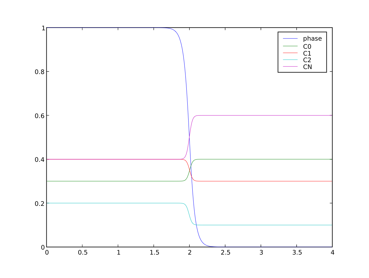
We can confirm that the far-field phases have remained separated

>>> X = mesh.faceCenters[0]
>>> print(numerix.allclose(phase.faceValue[X.value==0], 1.0, rtol = 1e-5, atol = 1e-5))
True
>>> print(numerix.allclose(phase.faceValue[X.value==L], 0.0, rtol = 1e-5, atol = 1e-5))
True

and that the concentration fields have appropriately segregated into their equilibrium values in each phase

>>> equilibrium = True
>>> for Cj in interstitials + substitutionals:
...     equilibrium &= numerix.allclose(Cj.faceValue[X.value==0], Cj.S, rtol = 3e-3, atol = 3e-3).value
...     equilibrium &= numerix.allclose(Cj.faceValue[X.value==L], Cj.L, rtol = 3e-3, atol = 3e-3).value
>>> print(equilibrium)
True

Last updated on Feb 14, 2025. Created using Sphinx 7.1.2.