examples.levelSet.electroChem.leveler¶

Model electrochemical superfill of copper with leveler and accelerator additives.

This input file is a demonstration of the use of FiPy for modeling copper superfill with leveler and accelerator additives. The material properties and experimental parameters used are roughly those that have been previously published [28].

To run this example from the base FiPy directory type:

$ python examples/levelSet/electroChem/leveler.py

at the command line. The results of the simulation will be displayed and the word finished in the terminal at the end of the simulation. The simulation will only run for 200 time steps. To run with a different number of time steps change the numberOfSteps argument as follows,

>>> runLeveler(numberOfSteps=10, displayViewers=False, cellSize=0.25e-7) 
1

Change the displayViewers argument to True if you wish to see the results displayed on the screen. This example requires gmsh to construct the mesh.

This example models the case when suppressor, accelerator and leveler additives are present in the electrolyte. The suppressor is assumed to absorb quickly compared with the other additives. Any unoccupied surface sites are immediately covered with suppressor. The accelerator additive has more surface affinity than suppressor and is thus preferential adsorbed. The accelerator can also remove suppressor when the surface reaches full coverage. Similarly, the leveler additive has more surface affinity than both the suppressor and accelerator. This forms a simple set of assumptions for understanding the behavior of these additives.

The following is a complete description of the equations for the model described here. Any equations that have been omitted are the same as those given in examples.levelSet.electroChem.simpleTrenchSystem. The current density is governed by

i = \frac{c_{m}}{c_{m}^{\infty}} \sum_{j} [i_{j} θ_{j} (\exp \frac{- α_{j} F η}{R T} - \exp \frac{(1 - α_{j}) F η}{R T})]

where $j$ represents $S$ for suppressor, $A$ for accelerator, $L$ for leveler and $V$ for vacant. This model assumes a linear interpolation between the three cases of complete coverage for each additive or vacant substrate. The governing equations for the surfactants are given by,

\begin{aligned} \dot{θ_{L}} & = κ v θ_{L} + k_{l}^{+} c_{L} (1 - θ_{L}) - k_{L}^{-} v θ_{L}, \\ \dot{θ_{a}} & = κ v θ_{A} + k_{A}^{+} c_{A} (1 - θ_{A} - θ_{L}) - k_{L} c_{L} θ_{A} - k_{A}^{-} θ_{A}^{q - 1}, \\ θ_{S} & = 1 - θ_{A} - θ_{L} \\ θ_{V} & = 0. \end{aligned}

It has been found experimentally that $i_{L} = i_{S}$ .

If the surface reaches full coverage, the equations do not naturally prevent the coverage rising above full coverage due to the curvature terms. Thus, when $θ_{L} + θ_{A} = 1$ then the equation for accelerator becomes $\dot{θ_{A}} = - \dot{θ_{L}}$ and when $θ_{L} = 1$ , the equation for leveler becomes $\dot{θ_{L}} = - k_{L}^{-} v θ_{L} .$

The parameters $k_{A}^{+}$ , $k_{A}^{-}$ and $q$ are both functions of $η$ given by,

\begin{aligned} k_{A}^{+} & = k_{A 0}^{+} \exp \frac{- α_{k} F η}{R T}, \\ k_{A}^{-} & = B_{d} + \frac{A}{\exp (B_{a} (η + V_{d}))} + \exp (B_{b} (η + V_{d})) \\ q & = m η + b . \end{aligned}

The following table shows the symbols used in the governing equations and their corresponding arguments for the runLeveler() function.

\begin{array}{r} \begin{tabular}{|rllr@{.}ll|}\hlineSymbol                & Description                       & Keyword Argument                      & \multicolumn{2}{l}{Value} & Unit                               \\hline\multicolumn{6}{|c|}{Deposition Rate Parameters}                                                                                                                   \\hline v & deposition rate                   &                                       & \multicolumn{2}{l}{}      & m s^{- 1} \ i_{A} & accelerator current density       & \texttt{i0Accelerator}                & \multicolumn{2}{l}{}      & A m^{- 2} \ i_{L} & leveler current density           & \texttt{i0Leveler}                    & \multicolumn{2}{l}{}      & A m^{- 2} \ Ω & molar volume                      & \texttt{molarVolume}                  & 7&1 \times 10^{- 6} & m^{3} mol^{- 1} \ n & ion charge                        & \texttt{charge}                       & \multicolumn{2}{c}{2}     &                                    \ F & Faraday's constant                & \texttt{faradaysConstant}             & 9&6 \times 10^{- 4} & C mol^{- 1} \ i_{0} & exchange current density          &                                       & \multicolumn{2}{l}{}      & A m^{- 2} \ α_{A} & accelerator transfer coefficient  & \texttt{alphaAccelerator}             & 0&4                       &                                    \ α_{S} & leveler transfer coefficient      & \texttt{alphaLeveler}                 & 0&5                       &                                    \ η & overpotential                     & \texttt{overpotential}                & -0&3                      & V                                  \ R & gas constant                      & \texttt{gasConstant}                  & 8&314                     & J K mol^{- 1} \ T & temperature                       & \texttt{temperature}                  & 298&0                     & K                                  \\hline\multicolumn{6}{|c|}{Ion Parameters}                                                                                                                               \\hline c_{I} & ion concentration                 & \texttt{ionConcentration}             & 250&0                     & mol m^{- 3} \ c_{I}^{\infty} & far field ion concentration       & \texttt{ionConcentration}             & 250&0                     & mol m^{- 3} \ D_{I} & ion diffusion coefficient         & \texttt{ionDiffusion}                 & 5&6 \times 10^{- 10} & m^{2} s^{- 1} \\hline\multicolumn{6}{|c|}{Accelerator Parameters}                                                                                                                       \\hline θ_{A} & accelerator coverage              & \texttt{acceleratorCoverage}          & 0&0                       &                                    \ c_{A} & accelerator concentration         & \texttt{acceleratorConcentration}     & 5&0 \times 10^{- 3} & mol m^{- 3} \ c_{A}^{\infty} & far field accelerator concentration & \texttt{acceleratorConcentration}   & 5&0 \times 10^{- 3} & mol m^{- 3} \ D_{A} & catalyst diffusion coefficient    & \texttt{catalystDiffusion}            & 1&0 \times 10^{- 9} & m^{2} s^{- 1} \ Γ_{A} & accelerator site density          & \texttt{siteDensity}                  & 9&8 \times 10^{- 6} & mol m^{- 2} \ k_{A}^{+} & accelerator adsorption            &                                       & \multicolumn{2}{l}{}      & m^{3} mol^{- 1} s^{- 1} \ k_{A 0}^{+} & accelerator adsorption coeff      & \texttt{kAccelerator0}                & 2&6 \times 10^{- 4} & m^{3} mol^{- 1} s^{- 1} \ α_{k} & accelerator adsorption coeff      & \texttt{alphaAdsorption}              & 0&62                      &                                    \ k_{A}^{-} & accelerator consumption coeff     &                                       & \multicolumn{2}{l}{}      &                                    \ B_{a} & experimental parameter            & \texttt{Bd}                           & -40&0                     &\ B_{b} & experimental parameter            & \texttt{Bd}                           & 60&0                      &\ V_{d} & experimental parameter            & \texttt{Bd}                           & 9&8 \times 10^{- 2} &\ B_{d} & experimental parameter            & \texttt{Bd}                           & 8&0 \times 10^{- 4} &\\hline\multicolumn{6}{|c|}{Geometry Parameters}                                                                                                                          \\hline D & trench depth                      & \texttt{trenchDepth}                  & 0&5 \times 10^{- 6} & m                                  \ D / W & trench aspect ratio               & \texttt{aspectRatio}                  & 2&0                       &                                    \ S & trench spacing                    & \texttt{trenchSpacing}                & 0&6 \times 10^{- 6} & m                                  \ δ & boundary layer depth              & \texttt{boundaryLayerDepth}           & 0&3 \times 10^{- 6} & m                                  \\hline\multicolumn{6}{|c|}{Simulation Control Parameters}                                                                                                                \\hline& computational cell size           & \texttt{cellSize}                     & 0&1 \times 10^{- 7} & m                                  \& number of time steps              & \texttt{numberOfSteps}                & \multicolumn{2}{c}{5}     &                                    \& whether to display the viewers    & \texttt{displayViewers}               & \multicolumn{2}{c}{\texttt{True}} &                           \\hline\end{tabular} \end{array}

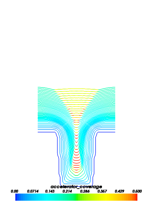
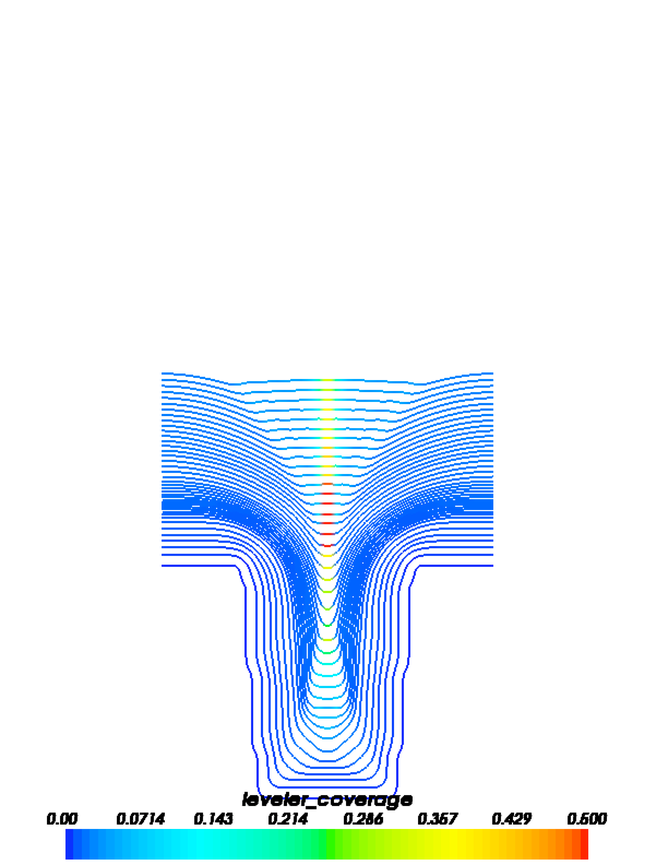
The following images show accelerator and leveler contour plots that can be obtained by running this example.

accelerator coverage as a function of time during superfill

leveler coverage as a function of time during superfill

Last updated on Feb 14, 2025. Created using Sphinx 7.1.2.

examples.levelSet.electroChem.leveler¶

Versions

Downloads

GitHub