fipy.variables.betaNoiseVariable¶

Classes

BetaNoiseVariable(*args, **kwds)

Represents a beta distribution of random numbers with the probability distribution

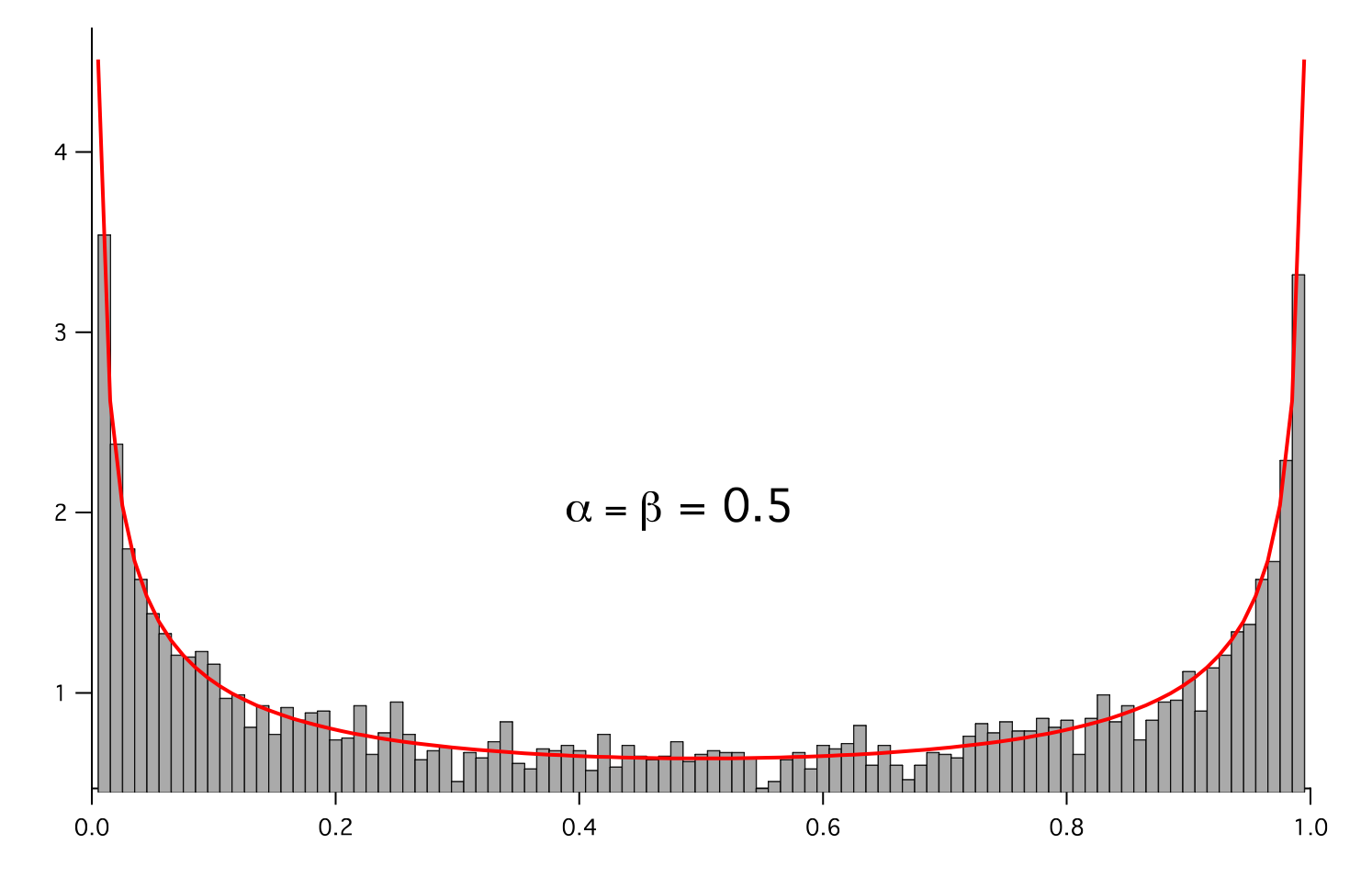
class fipy.variables.betaNoiseVariable.BetaNoiseVariable(*args, **kwds)¶

Bases: NoiseVariable

Represents a beta distribution of random numbers with the probability distribution

\[x^{\alpha - 1}\frac{\beta^\alpha e^{-\beta x}}{\Gamma(\alpha)}\]

with a shape parameter $\alpha$, a rate parameter $\beta$, and $\Gamma(z) = \int_0^\infty t^{z - 1}e^{-t}\,dt$.

Seed the random module for the sake of deterministic test results.

>>> from fipy import numerix
>>> numerix.random.seed(1)

We generate noise on a uniform Cartesian mesh

>>> from fipy.variables.variable import Variable
>>> alpha = Variable()
>>> beta = Variable()
>>> from fipy.meshes import Grid2D
>>> noise = BetaNoiseVariable(mesh = Grid2D(nx = 100, ny = 100), alpha = alpha, beta = beta)

We histogram the root-volume-weighted noise distribution

>>> from fipy.variables.histogramVariable import HistogramVariable
>>> histogram = HistogramVariable(distribution = noise, dx = 0.01, nx = 100)

and compare to a Gaussian distribution

>>> from fipy.variables.cellVariable import CellVariable
>>> betadist = CellVariable(mesh = histogram.mesh)
>>> x = CellVariable(mesh=histogram.mesh, value=histogram.mesh.cellCenters[0])
>>> from scipy.special import gamma as Gamma 
>>> betadist = ((Gamma(alpha + beta) / (Gamma(alpha) * Gamma(beta)))
...             * x**(alpha - 1) * (1 - x)**(beta - 1)) 

>>> if __name__ == '__main__':
...     from fipy import Viewer
...     viewer = Viewer(vars=noise, datamin=0, datamax=1)
...     histoplot = Viewer(vars=(histogram, betadist),
...                        datamin=0, datamax=1.5)

>>> from fipy.tools.numerix import arange

>>> for a in arange(0.5, 5, 0.5):
...     alpha.value = a
...     for b in arange(0.5, 5, 0.5):
...         beta.value = b
...         if __name__ == '__main__':
...             import sys
...             print("alpha: %g, beta: %g" % (alpha, beta), file=sys.stderr)
...             viewer.plot()
...             histoplot.plot()

>>> print(abs(noise.faceGrad.divergence.cellVolumeAverage) < 5e-15)
1

histogram of random values with a beta distribution

Parameters:

mesh (Mesh) – The mesh on which to define the noise.
alpha (float) – The parameter $\alpha$.
beta (float) – The parameter $\beta$.

__abs__()¶

Following test it to fix a bug with C inline string using abs() instead of fabs()

>>> print(abs(Variable(2.3) - Variable(1.2)))
1.1

Check representation works with different versions of numpy

>>> print(repr(abs(Variable(2.3))))
numerix.fabs(Variable(value=array(2.3)))

__and__(other)¶

This test case has been added due to a weird bug that was appearing.

>>> a = Variable(value=(0, 0, 1, 1))
>>> b = Variable(value=(0, 1, 0, 1))
>>> print(numerix.equal((a == 0) & (b == 1), [False,  True, False, False]).all())
True
>>> print(a & b)
[0 0 0 1]
>>> from fipy.meshes import Grid1D
>>> mesh = Grid1D(nx=4)
>>> from fipy.variables.cellVariable import CellVariable
>>> a = CellVariable(value=(0, 0, 1, 1), mesh=mesh)
>>> b = CellVariable(value=(0, 1, 0, 1), mesh=mesh)
>>> print(numerix.allequal((a == 0) & (b == 1), [False,  True, False, False]))
True
>>> print(a & b)
[0 0 0 1]

__array__(dtype=None, copy=None)¶

Attempt to convert the Variable to a numerix array object

>>> v = Variable(value=[2, 3])
>>> print(numerix.array(v))
[2 3]

A dimensional Variable will convert to the numeric value in its base units

>>> v = Variable(value=[2, 3], unit="mm")
>>> numerix.array(v)
array([ 0.002,  0.003])

__array_wrap__(arr, context=None, return_scalar=False)¶

Required to prevent numpy not calling the reverse binary operations. Both the following tests are examples ufuncs.

>>> print(type(numerix.array([1.0, 2.0]) * Variable([1.0, 2.0]))) 
<class 'fipy.variables.binaryOperatorVariable...binOp'>

>>> from scipy.special import gamma as Gamma 
>>> print(type(Gamma(Variable([1.0, 2.0])))) 
<class 'fipy.variables.unaryOperatorVariable...unOp'>

__bool__()¶

>>> print(bool(Variable(value=0)))
0
>>> print(bool(Variable(value=(0, 0, 1, 1))))
Traceback (most recent call last):
    ...
ValueError: The truth value of an array with more than one element is ambiguous. Use a.any() or a.all()

__call__(points=None, order=0, nearestCellIDs=None)¶

Interpolates the CellVariable to a set of points using a method that has a memory requirement on the order of Ncells by Npoints in general, but uses only Ncells when the CellVariable’s mesh is a UniformGrid object.

Tests

>>> from fipy import *
>>> m = Grid2D(nx=3, ny=2)
>>> v = CellVariable(mesh=m, value=m.cellCenters[0])
>>> print(v(((0., 1.1, 1.2), (0., 1., 1.))))
[ 0.5  1.5  1.5]
>>> print(v(((0., 1.1, 1.2), (0., 1., 1.)), order=1))
[ 0.25  1.1   1.2 ]
>>> m0 = Grid2D(nx=2, ny=2, dx=1., dy=1.)
>>> m1 = Grid2D(nx=4, ny=4, dx=.5, dy=.5)
>>> x, y = m0.cellCenters
>>> v0 = CellVariable(mesh=m0, value=x * y)
>>> print(v0(m1.cellCenters.globalValue))
[ 0.25  0.25  0.75  0.75  0.25  0.25  0.75  0.75  0.75  0.75  2.25  2.25
  0.75  0.75  2.25  2.25]
>>> print(v0(m1.cellCenters.globalValue, order=1))
[ 0.125  0.25   0.5    0.625  0.25   0.375  0.875  1.     0.5    0.875
  1.875  2.25   0.625  1.     2.25   2.625]

Parameters:

points (tuple or list of tuple) – A point or set of points in the format (X, Y, Z)
order ({0, 1}) – The order of interpolation, default is 0
nearestCellIDs (array_like) – Optional argument if user can calculate own nearest cell IDs array, shape should be same as points

__eq__(other)¶

Test if a Variable is equal to another quantity

>>> a = Variable(value=3)
>>> b = (a == 4)
>>> b
(Variable(value=array(3)) == 4)
>>> b()
0

__ge__(other)¶

Test if a Variable is greater than or equal to another quantity

>>> a = Variable(value=3)
>>> b = (a >= 4)
>>> b
(Variable(value=array(3)) >= 4)
>>> b()
0
>>> a.value = 4
>>> print(b())
1
>>> a.value = 5
>>> print(b())
1

__getitem__(index)¶

“Evaluate” the Variable and return the specified element

>>> a = Variable(value=((3., 4.), (5., 6.)), unit="m") + "4 m"
>>> print(a[1, 1])
10.0 m

It is an error to slice a Variable whose value is not sliceable

>>> Variable(value=3)[2]
Traceback (most recent call last):
      ...
IndexError: 0-d arrays can't be indexed

__getstate__()¶: Used internally to collect the necessary information to pickle the CellVariable to persistent storage.

__gt__(other)¶

Test if a Variable is greater than another quantity

>>> a = Variable(value=3)
>>> b = (a > 4)
>>> b
(Variable(value=array(3)) > 4)
>>> print(b())
0
>>> a.value = 5
>>> print(b())
1

__hash__()¶: Return hash(self).

__invert__()¶

Returns logical “not” of the Variable

>>> a = Variable(value=True)
>>> print(~a)
False

__le__(other)¶

Test if a Variable is less than or equal to another quantity

>>> a = Variable(value=3)
>>> b = (a <= 4)
>>> b
(Variable(value=array(3)) <= 4)
>>> b()
1
>>> a.value = 4
>>> print(b())
1
>>> a.value = 5
>>> print(b())
0

__lt__(other)¶

Test if a Variable is less than another quantity

>>> a = Variable(value=3)
>>> b = (a < 4)
>>> b
(Variable(value=array(3)) < 4)
>>> b()
1
>>> a.value = 4
>>> print(b())
0
>>> print(1000000000000000000 * Variable(1) < 1.)
0
>>> print(1000 * Variable(1) < 1.)
0

Python automatically reverses the arguments when necessary

>>> 4 > Variable(value=3)
(Variable(value=array(3)) < 4)

__ne__(other)¶

Test if a Variable is not equal to another quantity

>>> a = Variable(value=3)
>>> b = (a != 4)
>>> b
(Variable(value=array(3)) != 4)
>>> b()
1

static __new__(cls, *args, **kwds)¶

__nonzero__()¶

>>> print(bool(Variable(value=0)))
0
>>> print(bool(Variable(value=(0, 0, 1, 1))))
Traceback (most recent call last):
    ...
ValueError: The truth value of an array with more than one element is ambiguous. Use a.any() or a.all()

__or__(other)¶

This test case has been added due to a weird bug that was appearing.

>>> a = Variable(value=(0, 0, 1, 1))
>>> b = Variable(value=(0, 1, 0, 1))
>>> print(numerix.equal((a == 0) | (b == 1), [True,  True, False, True]).all())
True
>>> print(a | b)
[0 1 1 1]
>>> from fipy.meshes import Grid1D
>>> mesh = Grid1D(nx=4)
>>> from fipy.variables.cellVariable import CellVariable
>>> a = CellVariable(value=(0, 0, 1, 1), mesh=mesh)
>>> b = CellVariable(value=(0, 1, 0, 1), mesh=mesh)
>>> print(numerix.allequal((a == 0) | (b == 1), [True,  True, False, True]))
True
>>> print(a | b)
[0 1 1 1]

__pow__(other)¶

return self**other, or self raised to power other

>>> print(Variable(1, "mol/l")**3)
1.0 mol**3/l**3
>>> print((Variable(1, "mol/l")**3).unit)
<PhysicalUnit mol**3/l**3>

__repr__()¶: Return repr(self).

__setstate__(dict)¶: Used internally to create a new CellVariable from pickled persistent storage.

__str__()¶: Return str(self).

all(axis=None)¶

>>> print(Variable(value=(0, 0, 1, 1)).all())
0
>>> print(Variable(value=(1, 1, 1, 1)).all())
1

allclose(other, rtol=1e-05, atol=1e-08)¶

>>> var = Variable((1, 1))
>>> print(var.allclose((1, 1)))
1
>>> print(var.allclose((1,)))
1

The following test is to check that the system does not run out of memory.

>>> from fipy.tools import numerix
>>> var = Variable(numerix.ones(10000))
>>> print(var.allclose(numerix.zeros(10000, 'l')))
False

any(axis=None)¶

>>> print(Variable(value=0).any())
0
>>> print(Variable(value=(0, 0, 1, 1)).any())
1

property arithmeticFaceValue¶

Returns a FaceVariable whose value corresponds to the arithmetic interpolation of the adjacent cells:

\[\phi_f = (\phi_1 - \phi_2) \frac{d_{f2}}{d_{12}} + \phi_2\]

>>> from fipy.meshes import Grid1D
>>> from fipy import numerix
>>> mesh = Grid1D(dx = (1., 1.))
>>> L = 1
>>> R = 2
>>> var = CellVariable(mesh = mesh, value = (L, R))
>>> faceValue = var.arithmeticFaceValue[mesh.interiorFaces.value]
>>> answer = (R - L) * (0.5 / 1.) + L
>>> print(numerix.allclose(faceValue, answer, atol = 1e-10, rtol = 1e-10))
True

>>> mesh = Grid1D(dx = (2., 4.))
>>> var = CellVariable(mesh = mesh, value = (L, R))
>>> faceValue = var.arithmeticFaceValue[mesh.interiorFaces.value]
>>> answer = (R - L) * (1.0 / 3.0) + L
>>> print(numerix.allclose(faceValue, answer, atol = 1e-10, rtol = 1e-10))
True

>>> mesh = Grid1D(dx = (10., 100.))
>>> var = CellVariable(mesh = mesh, value = (L, R))
>>> faceValue = var.arithmeticFaceValue[mesh.interiorFaces.value]
>>> answer = (R - L) * (5.0 / 55.0) + L
>>> print(numerix.allclose(faceValue, answer, atol = 1e-10, rtol = 1e-10))
True

property cellVolumeAverage¶

Return the cell-volume-weighted average of the CellVariable:

\[<\phi>_\text{vol} = \frac{\sum_\text{cells} \phi_\text{cell} V_\text{cell}} {\sum_\text{cells} V_\text{cell}}\]

>>> from fipy.meshes import Grid2D
>>> from fipy.variables.cellVariable import CellVariable
>>> mesh = Grid2D(nx = 3, ny = 1, dx = .5, dy = .1)
>>> var = CellVariable(value = (1, 2, 6), mesh = mesh)
>>> print(var.cellVolumeAverage)
3.0

constrain(value, where=None)¶

Constrains the CellVariable to value at a location specified by where.

>>> from fipy import *
>>> m = Grid1D(nx=3)
>>> v = CellVariable(mesh=m, value=m.cellCenters[0])
>>> v.constrain(0., where=m.facesLeft)
>>> v.faceGrad.constrain([1.], where=m.facesRight)
>>> print(v.faceGrad)
[[ 1.  1.  1.  1.]]
>>> print(v.faceValue)
[ 0.   1.   2.   2.5]

Changing the constraint changes the dependencies

>>> v.constrain(1., where=m.facesLeft)
>>> print(v.faceGrad)
[[-1.  1.  1.  1.]]
>>> print(v.faceValue)
[ 1.   1.   2.   2.5]

Constraints can be Variable

>>> c = Variable(0.)
>>> v.constrain(c, where=m.facesLeft)
>>> print(v.faceGrad)
[[ 1.  1.  1.  1.]]
>>> print(v.faceValue)
[ 0.   1.   2.   2.5]
>>> c.value = 1.
>>> print(v.faceGrad)
[[-1.  1.  1.  1.]]
>>> print(v.faceValue)
[ 1.   1.   2.   2.5]

Constraints can have a Variable mask.

>>> v = CellVariable(mesh=m)
>>> mask = FaceVariable(mesh=m, value=m.facesLeft)
>>> v.constrain(1., where=mask)
>>> print(v.faceValue)
[ 1.  0.  0.  0.]
>>> mask[:] = mask | m.facesRight
>>> print(v.faceValue)
[ 1.  0.  0.  1.]

property constraintMask¶

Test that constraintMask returns a Variable that updates itself whenever the constraints change.

>>> from fipy import *

>>> m = Grid2D(nx=2, ny=2)
>>> x, y = m.cellCenters
>>> v0 = CellVariable(mesh=m)
>>> v0.constrain(1., where=m.facesLeft)
>>> print(v0.faceValue.constraintMask)
[False False False False False False  True False False  True False False]
>>> print(v0.faceValue)
[ 0.  0.  0.  0.  0.  0.  1.  0.  0.  1.  0.  0.]
>>> v0.constrain(3., where=m.facesRight)
>>> print(v0.faceValue.constraintMask)
[False False False False False False  True False  True  True False  True]
>>> print(v0.faceValue)
[ 0.  0.  0.  0.  0.  0.  1.  0.  3.  1.  0.  3.]
>>> v1 = CellVariable(mesh=m)
>>> v1.constrain(1., where=(x < 1) & (y < 1))
>>> print(v1.constraintMask)
[ True False False False]
>>> print(v1)
[ 1.  0.  0.  0.]
>>> v1.constrain(3., where=(x > 1) & (y > 1))
>>> print(v1.constraintMask)
[ True False False  True]
>>> print(v1)
[ 1.  0.  0.  3.]

copy()¶: Copy the value of the NoiseVariable to a static CellVariable.

dot(other, opShape=None, operatorClass=None)¶

Return the mesh-element–by–mesh-element (cell-by-cell, face-by-face, etc.) scalar product

\[ext{self} \cdot ext{other}\]

Both self and other can be of arbitrary rank, and other does not need to be a MeshVariable.

property dtype¶

Returns the Numpy dtype of the underlying array.

>>> issubclass(Variable(1).dtype.type, numerix.integer)
True
>>> issubclass(Variable(1.).dtype.type, numerix.floating)
True
>>> issubclass(Variable((1, 1.)).dtype.type, numerix.floating)
True

property faceGrad¶: Return $\nabla \phi$ as a rank-1 FaceVariable using differencing for the normal direction(second-order gradient).

property faceGradAverage¶: Deprecated since version 3.3: use grad.arithmeticFaceValue instead

Return $\nabla \phi$ as a rank-1 FaceVariable using averaging for the normal direction(second-order gradient)

property faceValue¶

Returns a FaceVariable whose value corresponds to the arithmetic interpolation of the adjacent cells:

\[\phi_f = (\phi_1 - \phi_2) \frac{d_{f2}}{d_{12}} + \phi_2\]

>>> from fipy.meshes import Grid1D
>>> from fipy import numerix
>>> mesh = Grid1D(dx = (1., 1.))
>>> L = 1
>>> R = 2
>>> var = CellVariable(mesh = mesh, value = (L, R))
>>> faceValue = var.arithmeticFaceValue[mesh.interiorFaces.value]
>>> answer = (R - L) * (0.5 / 1.) + L
>>> print(numerix.allclose(faceValue, answer, atol = 1e-10, rtol = 1e-10))
True

>>> mesh = Grid1D(dx = (2., 4.))
>>> var = CellVariable(mesh = mesh, value = (L, R))
>>> faceValue = var.arithmeticFaceValue[mesh.interiorFaces.value]
>>> answer = (R - L) * (1.0 / 3.0) + L
>>> print(numerix.allclose(faceValue, answer, atol = 1e-10, rtol = 1e-10))
True

>>> mesh = Grid1D(dx = (10., 100.))
>>> var = CellVariable(mesh = mesh, value = (L, R))
>>> faceValue = var.arithmeticFaceValue[mesh.interiorFaces.value]
>>> answer = (R - L) * (5.0 / 55.0) + L
>>> print(numerix.allclose(faceValue, answer, atol = 1e-10, rtol = 1e-10))
True

property gaussGrad¶: Return $\frac{1}{V_P} \sum_f \vec{n} \phi_f A_f$ as a rank-1 CellVariable (first-order gradient).

property globalValue¶

Concatenate and return values from all processors

When running on a single processor, the result is identical to value.

property grad¶: Return $\nabla \phi$ as a rank-1 CellVariable (first-order gradient).

property harmonicFaceValue¶

Returns a FaceVariable whose value corresponds to the harmonic interpolation of the adjacent cells:

\[\phi_f = \frac{\phi_1 \phi_2}{(\phi_2 - \phi_1) \frac{d_{f2}}{d_{12}} + \phi_1}\]

>>> from fipy.meshes import Grid1D
>>> from fipy import numerix
>>> mesh = Grid1D(dx = (1., 1.))
>>> L = 1
>>> R = 2
>>> var = CellVariable(mesh = mesh, value = (L, R))
>>> faceValue = var.harmonicFaceValue[mesh.interiorFaces.value]
>>> answer = L * R / ((R - L) * (0.5 / 1.) + L)
>>> print(numerix.allclose(faceValue, answer, atol = 1e-10, rtol = 1e-10))
True

>>> mesh = Grid1D(dx = (2., 4.))
>>> var = CellVariable(mesh = mesh, value = (L, R))
>>> faceValue = var.harmonicFaceValue[mesh.interiorFaces.value]
>>> answer = L * R / ((R - L) * (1.0 / 3.0) + L)
>>> print(numerix.allclose(faceValue, answer, atol = 1e-10, rtol = 1e-10))
True

>>> mesh = Grid1D(dx = (10., 100.))
>>> var = CellVariable(mesh = mesh, value = (L, R))
>>> faceValue = var.harmonicFaceValue[mesh.interiorFaces.value]
>>> answer = L * R / ((R - L) * (5.0 / 55.0) + L)
>>> print(numerix.allclose(faceValue, answer, atol = 1e-10, rtol = 1e-10))
True

inBaseUnits()¶

Return the value of the Variable with all units reduced to their base SI elements.

>>> e = Variable(value="2.7 Hartree*Nav")
>>> print(e.inBaseUnits().allclose("7088849.01085 kg*m**2/s**2/mol"))
1

inUnitsOf(*units)¶

Returns one or more Variable objects that express the same physical quantity in different units. The units are specified by strings containing their names. The units must be compatible with the unit of the object. If one unit is specified, the return value is a single Variable.

>>> freeze = Variable('0 degC')
>>> print(freeze.inUnitsOf('degF').allclose("32.0 degF"))
1

If several units are specified, the return value is a tuple of Variable instances with with one element per unit such that the sum of all quantities in the tuple equals the the original quantity and all the values except for the last one are integers. This is used to convert to irregular unit systems like hour/minute/second. The original object will not be changed.

>>> t = Variable(value=314159., unit='s')
>>> from builtins import zip
>>> print(numerix.allclose([e.allclose(v) for (e, v) in zip(t.inUnitsOf('d', 'h', 'min', 's'),
...                                                         ['3.0 d', '15.0 h', '15.0 min', '59.0 s'])],
...                        True))
1

property leastSquaresGrad¶

Return $\nabla \phi$, which is determined by solving for $\nabla \phi$ in the following matrix equation,

\[\nabla \phi \cdot \sum_f d_{AP}^2 \vec{n}_{AP} \otimes \vec{n}_{AP} = \sum_f d_{AP}^2 \left( \vec{n} \cdot \nabla \phi \right)_{AP}\]

The matrix equation is derived by minimizing the following least squares sum,

\[F \left( \phi_x, \phi_y \right) = \sqrt{\sum_f \left( d_{AP} \vec{n}_{AP} \cdot \nabla \phi - d_{AP} \left( \vec{n}_{AP} \cdot \nabla \phi \right)_{AP} \right)^2 }\]

Tests

>>> from fipy import Grid2D
>>> m = Grid2D(nx=2, ny=2, dx=0.1, dy=2.0)
>>> print(numerix.allclose(CellVariable(mesh=m, value=(0, 1, 3, 6)).leastSquaresGrad.globalValue, \
...                                     [[8.0, 8.0, 24.0, 24.0],
...                                      [1.2, 2.0, 1.2, 2.0]]))
True

>>> from fipy import Grid1D
>>> print(numerix.allclose(CellVariable(mesh=Grid1D(dx=(2.0, 1.0, 0.5)),
...                                     value=(0, 1, 2)).leastSquaresGrad.globalValue, [[0.461538461538, 0.8, 1.2]]))
True

property mag¶: The magnitude of the Variable, e.g., $|\vec{\psi}| = \sqrt{\vec{\psi}\cdot\vec{\psi}}$.

max(axis=None)¶: Return the maximum along a given axis.

min(axis=None)¶

>>> from fipy import Grid2D, CellVariable
>>> mesh = Grid2D(nx=5, ny=5)
>>> x, y = mesh.cellCenters
>>> v = CellVariable(mesh=mesh, value=x*y)
>>> print(v.min())
0.25

property minmodFaceValue¶

Returns a FaceVariable with a value that is the minimum of the absolute values of the adjacent cells. If the values are of opposite sign then the result is zero:

\[\begin{split}\phi_f = \begin{cases} \phi_1& \text{when $|\phi_1| \le |\phi_2|$},\\ \phi_2& \text{when $|\phi_2| < |\phi_1|$},\\ 0 & \text{when $\phi1 \phi2 < 0$} \end{cases}\end{split}\]

>>> from fipy import *
>>> print(CellVariable(mesh=Grid1D(nx=2), value=(1, 2)).minmodFaceValue)
[1 1 2]
>>> print(CellVariable(mesh=Grid1D(nx=2), value=(-1, -2)).minmodFaceValue)
[-1 -1 -2]
>>> print(CellVariable(mesh=Grid1D(nx=2), value=(-1, 2)).minmodFaceValue)
[-1  0  2]

property old¶

Return the values of the CellVariable from the previous solution sweep.

Combinations of CellVariable’s should also return old values.

>>> from fipy.meshes import Grid1D
>>> mesh = Grid1D(nx = 2)
>>> from fipy.variables.cellVariable import CellVariable
>>> var1 = CellVariable(mesh = mesh, value = (2, 3), hasOld = 1)
>>> var2 = CellVariable(mesh = mesh, value = (3, 4))
>>> v = var1 * var2
>>> print(v)
[ 6 12]
>>> var1.value = ((3, 2))
>>> print(v)
[9 8]
>>> print(v.old)
[ 6 12]

The following small test is to correct for a bug when the operator does not just use variables.

>>> v1 = var1 * 3
>>> print(v1)
[9 6]
>>> print(v1.old)
[6 9]

rdot(other, opShape=None, operatorClass=None)¶

Return the mesh-element–by–mesh-element (cell-by-cell, face-by-face, etc.) scalar product

\[ext{other} \cdot ext{self}\]

Both self and other can be of arbitrary rank, and other does not need to be a MeshVariable.

release(constraint)¶

Remove constraint from self

>>> from fipy import *
>>> m = Grid1D(nx=3)
>>> v = CellVariable(mesh=m, value=m.cellCenters[0])
>>> c = Constraint(0., where=m.facesLeft)
>>> v.constrain(c)
>>> print(v.faceValue)
[ 0.   1.   2.   2.5]
>>> v.release(constraint=c)
>>> print(v.faceValue)
[ 0.5  1.   2.   2.5]

scramble()¶: Generate a new random distribution.

setValue(value, unit=None, where=None)¶

Set the value of the Variable. Can take a masked array.

>>> a = Variable((1, 2, 3))
>>> a.setValue(5, where=(1, 0, 1))
>>> print(a)
[5 2 5]

>>> b = Variable((4, 5, 6))
>>> a.setValue(b, where=(1, 0, 1))
>>> print(a)
[4 2 6]
>>> print(b)
[4 5 6]
>>> a.value = 3
>>> print(a)
[3 3 3]

>>> b = numerix.array((3, 4, 5))
>>> a.value = b
>>> a[:] = 1
>>> print(b)
[3 4 5]

>>> a.setValue((4, 5, 6), where=(1, 0)) 
Traceback (most recent call last):
    ....
ValueError: shape mismatch: objects cannot be broadcast to a single shape

property shape¶

>>> from fipy.meshes import Grid2D
>>> from fipy.variables.cellVariable import CellVariable
>>> mesh = Grid2D(nx=2, ny=3)
>>> var = CellVariable(mesh=mesh)
>>> print(numerix.allequal(var.shape, (6,))) 
True
>>> print(numerix.allequal(var.arithmeticFaceValue.shape, (17,))) 
True
>>> print(numerix.allequal(var.grad.shape, (2, 6))) 
True
>>> print(numerix.allequal(var.faceGrad.shape, (2, 17))) 
True

Have to account for zero length arrays

>>> from fipy import Grid1D
>>> m = Grid1D(nx=0)
>>> v = CellVariable(mesh=m, elementshape=(2,))
>>> numerix.allequal((v * 1).shape, (2, 0))
True

std(axis=None, **kwargs)¶

Evaluate standard deviation of all the elements of a MeshVariable.

Adapted from http://mpitutorial.com/tutorials/mpi-reduce-and-allreduce/

>>> import fipy as fp
>>> mesh = fp.Grid2D(nx=2, ny=2, dx=2., dy=5.)
>>> var = fp.CellVariable(value=(1., 2., 3., 4.), mesh=mesh)
>>> print((var.std()**2).allclose(1.25))
True

property unit¶

Return the unit object of self.

>>> Variable(value="1 m").unit
<PhysicalUnit m>

updateOld()¶

Set the values of the previous solution sweep to the current values.

>>> from fipy import *
>>> v = CellVariable(mesh=Grid1D(), hasOld=False)
>>> v.updateOld()
Traceback (most recent call last):
   ...
AssertionError: The updateOld method requires the CellVariable to have an old value. Set hasOld to True when instantiating the CellVariable.

property value¶

“Evaluate” the Variable and return its value (longhand)

>>> a = Variable(value=3)
>>> print(a.value)
3
>>> b = a + 4
>>> b
(Variable(value=array(3)) + 4)
>>> b.value
7

Last updated on Jun 26, 2024. Created using Sphinx 7.1.2.