examples.levelSet.electroChem.simpleTrenchSystem

Model electrochemical superfill using the CEAC mechanism.

This input file is a demonstration of the use of FiPy for modeling electrodeposition using the CEAC mechanism. The material properties and experimental parameters used are roughly those that have been previously published [29].

To run this example from the base FiPy directory type:

$ python examples/levelSet/electroChem/simpleTrenchSystem.py

at the command line. The results of the simulation will be displayed and the word finished in the terminal at the end of the simulation. To run with a different number of time steps change the numberOfSteps argument as follows,

>>> runSimpleTrenchSystem(numberOfSteps=2, displayViewers=False) 
1

Change the displayViewers argument to True if you wish to see the results displayed on the screen. Example examples.levelSet.electroChem.simpleTrenchSystem gives explanation for writing new scripts or modifying existing scripts that are encapsulated by functions.

Any argument parameter can be changed. For example if the initial catalyst coverage is not 0, then it can be reset,

>>> runSimpleTrenchSystem(numberOfSteps=2, catalystCoverage=0.1, displayViewers=False)
0

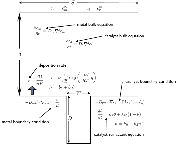
The following image shows a schematic of a trench geometry along with the governing equations for modeling electrodeposition with the CEAC mechanism. All of the given equations are implemented in the examples.levelSet.electroChem.simpleTrenchSystem.runSimpleTrenchSystem() function. As stated above, all the parameters in the equations can be changed with function arguments.

The following table shows the symbols used in the governing equations and their corresponding arguments to the runSimpleTrenchSystem() function. The boundary layer depth is intentionally small in this example in order not to complicate the mesh. Further examples will simulate more realistic boundary layer depths but will also have more complex meshes requiring the gmsh software.

\[\begin{split}\mbox{ \begin{tabular}{|rllr@{.}ll|} \hline Symbol & Description & Keyword Argument & \multicolumn{2}{l}{Value} & Unit \\ \hline \multicolumn{6}{|c|}{Deposition Rate Parameters} \\ \hline $v$ & deposition rate & & \multicolumn{2}{l}{} & m s$^{-1}$ \\ $i$ & current density & & \multicolumn{2}{l}{} & A m$^{-2}$ \\ $\Omega$ & molar volume & \texttt{molarVolume} & 7&1$\times$10$^{-6}$ & m$^3$ mol$^{-1}$ \\ $n$ & ion charge & \texttt{charge} & \multicolumn{2}{c}{2} & \\ $F$ & Faraday's constant & \texttt{faradaysConstant} & 9&6$\times$10$^{-4}$ & C mol$^{-1}$ \\ $i_0$ & exchange current density & & \multicolumn{2}{l}{} & A m$^{-2}$ \\ $\alpha$ & transfer coefficient & \texttt{transferCoefficient} & 0&5 & \\ $\eta$ & overpotential & \texttt{overpotential} & -0&3 & V \\ $R$ & gas constant & \texttt{gasConstant} & 8&314 & J K$^{-1}$ mol$^{-1}$ \\ $T$ & temperature & \texttt{temperature} & 298&0 & K \\ $b_0$ & current density for $\theta^0$ & \texttt{currentDensity0} & 0&26 & A m$^{-2}$ \\ $b_1$ & current density for $\theta$ & \texttt{currentDensity1} & 45&0 & A m$^{-2}$ \\ \hline \multicolumn{6}{|c|}{Metal Ion Parameters} \\ \hline $c_m$ & metal ion concentration & \texttt{metalConcentration} & 250&0 & mol m$^{-3}$ \\ $c_m^{\infty}$ & far field metal ion concentration & \texttt{metalConcentration} & 250&0 & mol m$^{-3}$ \\ $D_m$ & metal ion diffusion coefficient & \texttt{metalDiffusion} & 5&6$\times$10$^{-10}$ & m$^2$ s$^{-1}$ \\ \hline \multicolumn{6}{|c|}{Catalyst Parameters} \\ \hline $\theta$ & catalyst surfactant concentration & \texttt{catalystCoverage} & 0&0 & \\ $c_{\theta}$ & bulk catalyst concentration & \texttt{catalystConcentration} & 5&0$\times$10$^{-3}$ & mol m$^{-3}$ \\ $c_{\theta}^{\infty}$ & far field catalyst concentration & \texttt{catalystConcentration} & 5&0$\times$10$^{-3}$ & mol m$^{-3}$ \\ $D_{\theta}$ & catalyst diffusion coefficient & \texttt{catalystDiffusion} & 1&0$\times$10$^{-9}$ & m$^2$ s$^{-1}$ \\ $\Gamma$ & catalyst site density & \texttt{siteDensity} & 9&8$\times$10$^{-6}$ & mol m$^{-2}$ \\ $k$ & rate constant & & \multicolumn{2}{l}{} & m$^3$ mol$^{-1}$ s$^{-1}$ \\ $k_0$ & rate constant for $\eta^0$ & \texttt{rateConstant0} & 1&76 & m$^3$ mol$^{-1}$ s$^{-1}$ \\ $k_3$ & rate constant for $\eta^3$ & \texttt{rateConstant3} & -245&0$\times$10$^{-6}$ & m$^3$ mol$^{-1}$ s$^{-1}$ V$^{-3}$ \\ \hline \multicolumn{6}{|c|}{Geometry Parameters} \\ \hline $D$ & trench depth & \texttt{trenchDepth} & 0&5$\times$10$^{-6}$ & m \\ $D / W$ & trench aspect ratio & \texttt{aspectRatio} & 2&0 & \\ $S$ & trench spacing & \texttt{trenchSpacing} & 0&6$\times$10$^{-6}$ & m \\ $\delta$ & boundary layer depth & \texttt{boundaryLayerDepth} & 0&3$\times$10$^{-6}$ & m \\ \hline \multicolumn{6}{|c|}{Simulation Control Parameters} \\ \hline & computational cell size & \texttt{cellSize} & 0&1$\times$10$^{-7}$ & m \\ & number of time steps & \texttt{numberOfSteps} & \multicolumn{2}{c}{5} & \\ & whether to display the viewers & \texttt{displayViewers} & \multicolumn{2}{c}{\texttt{True}} & \\ \hline \end{tabular} }\end{split}\]

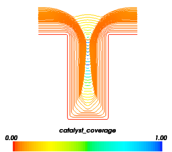
If the Mayavi plotting software is installed (see Installation) then a plot should appear that is updated every 20 time steps and will eventually resemble the image below.

Last updated on Nov 20, 2024. Created using Sphinx 7.1.2.