Solvers

FiPy requires either PETSc, pyamgx, Pysparse, SciPy, or Trilinos solver suites to be installed in order to solve linear systems. PETSc and Trilinos are the most complete of the solvers due to their numerous preconditioning and solver capabilities and they also allow FiPy to run in parallel. The Python interface for PETSc is better maintained than for Trilinos and tends to be easier to install. The sparse linear algebra solvers from the popular SciPy package are widely available and easy to install. Although they do not perform as well as the other suites and lack many of the features of PETSc or Trilinos, they may be the easiest linear solver choice when first installing and testing FiPy. While the Pysparse linear solvers offer a modest advantage in serial, be aware that they require Python 2.7, which is no longer supported. FiPy support for Pysparse will be dropped soon. pyamgx offers the possibility of solving sparse linear systems on the GPU; be aware that both hardware and software configuration is non-trivial.

FiPy chooses the solver suite based on system availability or based on the user supplied Command-line Flags and Environment Variables. For example, passing --no-pysparse:

$ python -c "from fipy import *; print DefaultSolver" --no-pysparse
<class 'fipy.solvers.trilinos.linearGMRESSolver.LinearGMRESSolver'>

uses a Trilinos solver. Setting FIPY_SOLVERS to scipy:

$ FIPY_SOLVERS=scipy
$ python -c "from fipy import *; print DefaultSolver"
<class 'fipy.solvers.scipy.linearLUSolver.LinearLUSolver'>

uses a SciPy solver. Suite-specific solver classes can also be imported and instantiated overriding any other directives. For example:

$ python -c "from fipy.solvers.scipy import DefaultSolver; \
>   print DefaultSolver" --no-pysparse
<class 'fipy.solvers.scipy.linearLUSolver.LinearLUSolver'>

uses a SciPy solver regardless of the command line argument. In the absence of Command-line Flags and Environment Variables, FiPy’s order of precedence when choosing the solver suite for generic solvers is PySparse followed by PETSc, Trilinos, SciPy, and pyamgx.

Solver Suite Features

	PETSc	PyAMG	pyamgx	Pysparse	SciPy	Trilinos
FIPY_SOLVERS	petsc		pyamgx	pysparse	scipy	trilinos or no-pysparse
solvers	✓		✓	✓	✓	✓
preconditioners	✓	✓	✓	✓	✓	✓
parallel	✓		[1]			✓
linux	✓	✓	✓	✓	✓	✓
macOS	✓	✓		✓	✓	✓
Windows		✓		✓	✓
requirements	petsc4py, mpi4py	pyamg, scipy	pyamgx, scipy, python >= 2.7 or >= 3.5	pysparse >= 1.0, python < 3	scipy	PyTrilinos, mpi4py, python >=3.7,<3.9 [2] [3], (pysparse [4])

[1]

While AMGX matrix solve takes advantage of GPU parallelism, the pyamgx library uses SciPy to build the matrix and thus suffers a significant serial bottleneck.

[2]

PyTrilinos may be compatible with newer versions of Python, but these are the most recent versions we’ve been able to get to install using conda (3.7 on linux and 3.8 on macOS).

[3]

There is a more actively developed PyTrilinos2 package, which may be compable with more recent versions of Python, but FiPy does not yet work with it.

[4]

Trilinos parallel efficiency is somewhat improved by also installing pysparse.

Note

FiPy has not been designed to mix different solver suites during a given problem run

PETSc

https://www.mcs.anl.gov/petsc

PETSc (the Portable, Extensible Toolkit for Scientific Computation) is a suite of data structures and routines for the scalable (parallel) solution of scientific applications modeled by partial differential equations. It employs the MPI standard for all message-passing communication (see Solving in Parallel for more details).

PyAMG

https://pyamg.readthedocs.io/

The PyAMG package provides adaptive multigrid preconditioners that can be used in conjunction with the SciPy solvers. While PyAMG also has solvers, they are not currently implemented in FiPy.

pyamgx

https://pyamgx.readthedocs.io/

The pyamgx package is a Python interface to the NVIDIA AMGX library. pyamgx can be used to construct complex solvers and preconditioners to solve sparse sparse linear systems on the GPU.

Pysparse

http://pysparse.sourceforge.net

Pysparse is a fast serial sparse matrix library for Python. It provides several sparse matrix storage formats and conversion methods. It also implements a number of iterative solvers, preconditioners, and interfaces to efficient factorization packages. The only requirement to install and use Pysparse is NumPy.

Warning

Pysparse is archaic and limited to Running under Python 2. Support for Python 2.7 and, thus, for Pysparse will be dropped soon.

SciPy

https://docs.scipy.org/doc/scipy/reference/sparse.html

The scipy.sparse module provides a basic set of serial Krylov solvers and a limited collection of preconditioners.

Trilinos

https://trilinos.github.io/

Trilinos provides a complete set of sparse matrices, solvers, and preconditioners. Trilinos preconditioning allows for iterative solutions to some difficult problems, and it enables parallel execution of FiPy (see Solving in Parallel for more details).

Performance Comparison

Comparing different solver suites, or even different solvers, has historically been difficult. The different suites have different interpretations of Convergence and tolerance. FiPy 4.0 harmonizes the different suites so that, to the greatest extent possible, all interpret Convergence and tolerance the same way. In the course of doing this, a number of inefficiencies were found in the way that FiPy built sparse matrices. To see the impact of these changes, we examine the serial and parallel scaling performance of the different solver suites for two different benchmark problems.

Serial Performance

Serial performance is compared for the different suites.

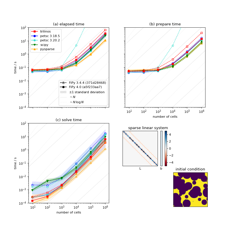
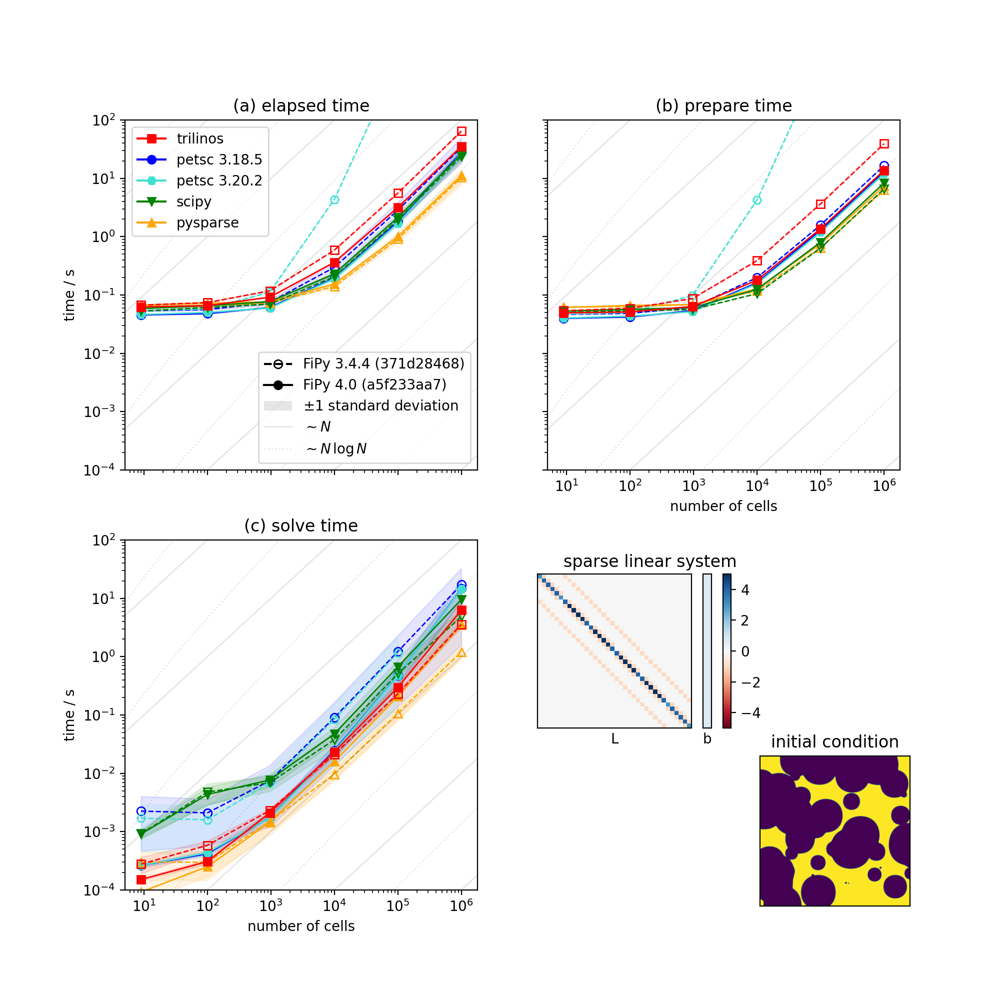
The following plot shows the serial scaling behavior for the different solvers. We compare solution time vs number mesh cells for a diffusion problem.

(Source code, png, hires.png, pdf)

Comparison of serial performance for different solver suites, solvers and preconditioners, and different versions of FiPy [5]. (a) Total elapsed time, (b) time to prepare the matrix, and (c) time to solve the matrix as functions of mesh size. [6]

We can see:

• For sufficiently large problems, building the matrix can be expected to scale as the number of cells \(N\) and solving the matrix should scale as \(N\,\ln N\). There are not enough data points to differentiate these slopes.

• Below about 1000 cells, the time to prepare the matrix is insensitive to mesh size and this dominates the overall elapsed time.

• There is nearly three orders of magnitude between the fastest solver/preconditioner and the slowest. This particular problem is not especially sensitive to choice of solver and preconditioner, as preparing the matrix takes the majority of the overall time, but it can be worth optimizing the choice for more complex systems of equations.

• Matrix preparation time is terrible when older FiPy is combined with newer PETSc. PETSc 3.19 introduced changes to “provide reasonable performance when no preallocation information is provided”. Our experience is opposite that; FiPy did not supply preallocation information prior to version 4.0, but matrix preparation performance was fine with older PETSc releases. FiPy 4.0 does supply preallocation information and matrix preparation time is comparable for all tested versions of PETSc.

• There is considerable dispersion about the mean solve time for different solvers and preconditioners. On the other hand, the time to prepare the matrix is insensitive to the choice of solver and preconditioner and shows a high degree of consistency from run to run.

(Source code, png, hires.png, pdf)

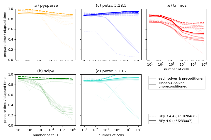
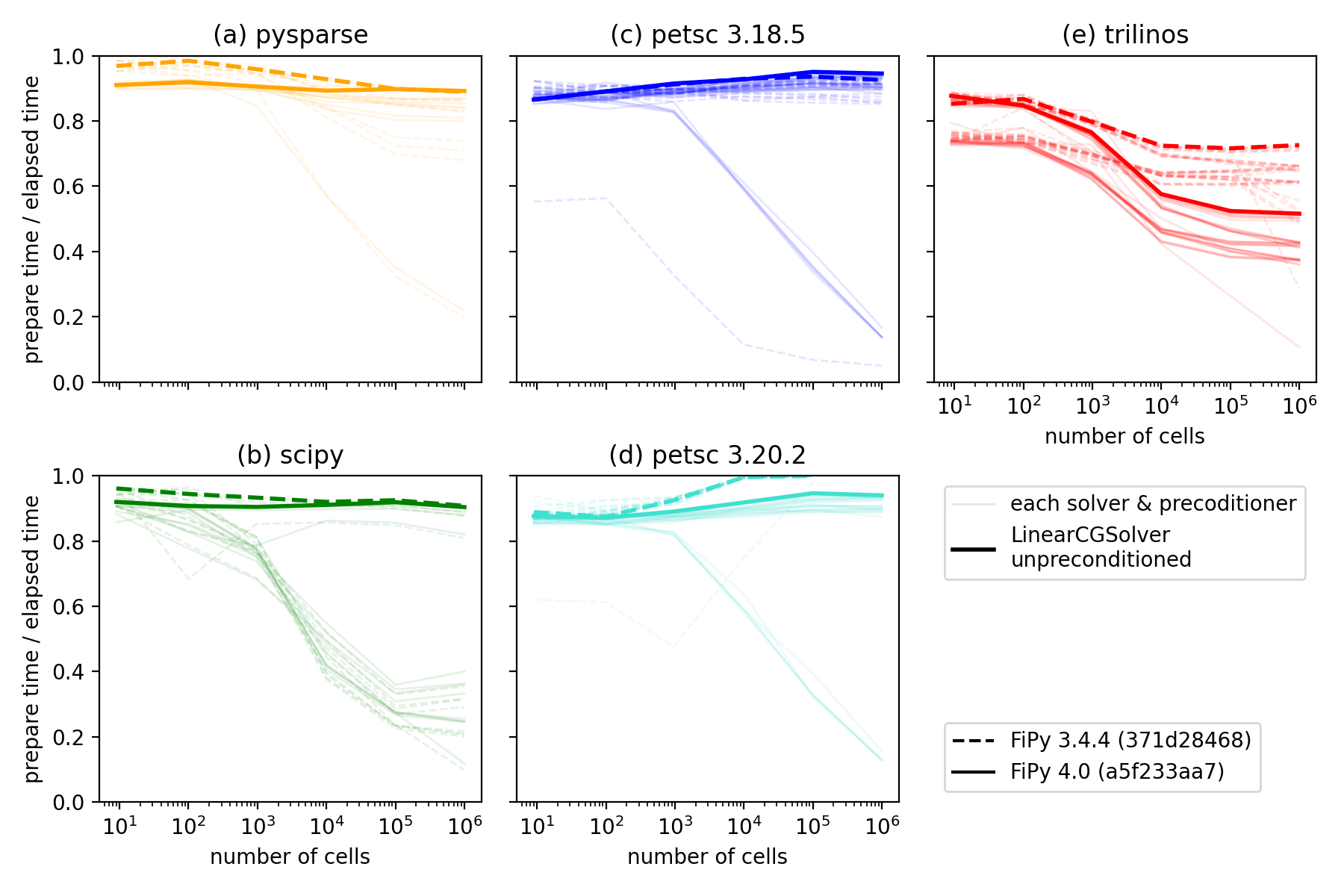
Ratio of time to prepare the matrix to the combined time to prepare and solve the matrix for different solver suites, solvers and preconditioners, and different versions of FiPy [5] [6]. The thick lines highlight LinearCGSolver with no preconditioner, one of the better-performing combinations available in all suites.

In principle, we’d like to spend as little time preparing the matrix, relative to solving it, as possible. This metric can be deceptive. If we compare the case of unpreconditioned LinearCGSolver, one of the fastest combinations for all suites for this problem, we see that Trilinos has the lowest ratio of prepare to elapsed time. Examination of elapsed time, the quantity we really care about, shows that Trilinos takes three times as long to both prepare and solve as Pysparse or SciPy and twice as long as PETSc.

For your own work, focus on identifying the solver and preconditioner with the lowest overall time to build and solve; this will counterintuitively have the highest ratio of prepare-to-elapsed time. Prepare time to elapsed time is a more useful metric for the FiPy developers; just as FiPy 4.0 brought considerable reductions in matrix build time, we will continue to seek opportunities to optimize.

Parallel Performance

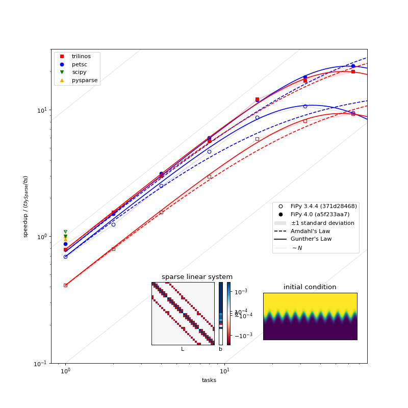
The following plot shows the scaling behavior for multiple processors. We compare solution time vs number of Slurm tasks (available cores) for a Method of Manufactured Solutions Allen-Cahn problem.

(Source code, png, hires.png, pdf)

Parallel scaling behavior of different solver packages and different versions of FiPy [5] [7].

A few things can be observed in this plot:

• PETSc, Pysparse, Trilinos, and SciPy have comparable serial performance, with SciPy edging out the other three for this particular problem.

• FiPy 4.0 is roughly the same speed in serial, but more than twice as fast in parallel compared to FiPy 3.4.4 when using the PETSc solvers. FiPy 4.0 is roughly twice as fast using the Trilinos solvers, whether in serial or parallel.

• FiPy 4.0 exhibits better parallel scaling than FiPy 3.4.4. Amdahl’s Law, \(\text{speedup} = p / (1 + \sigma(p - 1))\), does not fit the performance data nearly as well as Gunther’s Law, \(\text{speedup} = p / (1 + \sigma(p - 1) + \kappa p (p-1))\), where \(p\) is the number of parallel tasks, \(\sigma\) is the fraction limited by serial processes, and \(\kappa\) is “coherency” (which is somewhat nebulous).

  Parallel scaling fitting parameters (smaller numbers are better)

  		Amdahl	Gunther
  		serial / %	serial / %	coherency
  FiPy 3.4.4	petsc	4.7(3)	0.91(9)	0.00078(2)
  	trilinos	2.6(1)	0.8(1)	0.00034(2)
  FiPy 4.0	petsc	1.70(8)	0.13(7)	0.00028(1)
  	trilinos	2.2(1)	0.4(1)	0.00032(3)

At least one source of less-than-optimal scaling is that our “...Grid...” meshes parallelize by dividing the mesh into slabs, which leads to more communication overhead than more compact partitions. The “...Gmsh...” meshes partition more efficiently, but carry more overhead in other ways. We’ll be making efforts to improve the partitioning of the “...Grid...” meshes in a future release.

These results are likely both problem and architecture dependent. You should develop an understanding of the scaling behavior of your own codes before doing “production” runs.

[5] (1,2,3,4,5,6)

FiPy version 3.4.4 has different interpretations of Convergence for different solver suites (and even for different solvers). Benchmarks used a patched version (371d28468) that provided more logging information and normalized interpretation of tolerance, but without any of the improvements in matrix and solver efficiency of version 4.0.

[6] (1,2,3,4)

Calculations are of diffusion of a binary alloy in a frozen two-phase field. Solutions are on a square Grid2D. The initial condition is sampled from the center of a well-evolved \(1024\times 1024\) nucleation simulation. All available solvers and preconditioners are attempted. Solution tolerance is 1e-10 using the "RHS" convergence criterion. Simulations were run on an AMD Epyc 7702 CPU with 64 cores featuring two-thread Simultaneous Multi-Threading (SMT) and 512 GB of memory. OMP_NUM_THREADS was set to 1.

[7] (1,2)

Calculations are of a Method of Manufactured Solutions Allen-Cahn problem. Solutions are on a \(2048\times 1024\) Grid2D and the LinearCGSolver with no preconditioner is used for all solver suites. Solution tolerance is 1e-10 using the "RHS" convergence criterion. Five replicates of each simulation were run on an AMD Epyc 7702 CPU with 64 cores featuring two-thread Simultaneous Multi-Threading (SMT) and 512 GB of memory. OMP_NUM_THREADS was set to 1.

Convergence

Different solver suites take different approaches to testing convergence. We endeavor to harmonize this behavior by allowing the strings in the “criterion” column to be passed as an argument when instantiating a Solver. Convergence is detected if residual < tolerance * scale.

Residual Criteria

criterion	residual	scale	PETSc [8]	pyamgx [9]	PySparse	SciPy [10]	Trilinos [11]
unscaled	\(\|\mathsf{L}\vec{x} - \vec{b}\|_2\)	\(1\)	[12]	ABSOLUTE	[12]	[12]	AZ_noscaled
RHS	\(\|\mathsf{L}\vec{x} - \vec{b}\|_2\)	\(\|\vec{b}\|_2\)	KSP_NORM_UNPRECONDITIONED	[12]	cgs, pcg, qmres, or [12]	default	AZ_rhs
matrix	\(\|\mathsf{L}\vec{x} - \vec{b}\|_2\)	\(\|\mathsf{L}\|_\infty\)	[12]	[12]	[12]	[12]	AZ_Anorm
initial	\(\|\mathsf{L}\vec{x} - \vec{b}\|_2\)	\(\|\mathsf{L}\vec{x} - \vec{b}\|_2^{(0)}\)	[12]	RELATIVE_INI_CORE	bicgstab, gmres, minres, or [12]	[12]	AZ_r0
solution	\(\|\mathsf{L}\vec{x} - \vec{b}\|_\infty\)	\(\|\mathsf{L}\|_\infty * \|\vec{x}\|_1 + \|\vec{b}\|_\infty\)					AZ_sol
preconditioned	\(\left\|\mathsf{P}^{-1}(\mathsf{L}\vec{x} - \vec{b})\right\|_2\)	\(\left\|\vec{b}\right\|_2\)	KSP_NORM_PRECONDITIONED
natural	\(\sqrt{(\mathsf{L}\vec{x} - \vec{b})\mathsf{P}^{-1}(\mathsf{L}\vec{x} - \vec{b})}\)	\(\left\|\vec{b}\right\|_2\)	KSP_NORM_NATURAL
legacy			KSP_NORM_DEFAULT (RHS or preconditioned)	initial	RHS or initial	RHS	initial
default			RHS	RHS	RHS	RHS	RHS

Note

PyAMG is a set of preconditioners applied on top of SciPy, so is not explicitly included in these tables.

Tolerance

The default tolerance is \(10^{-5}\) (the legacy tolerance, prior to FiPy 4.0, was \(10^{-10}\)).

• SciPy and Trilinos can fail with tolerance=1e-10. (SCIPY_MAXIT or AZ_loss, respectively) because they are unable to make the residual any smaller than \(\mathcal{O}(10^{-9})\).

• tolerance=1e-5 is the default for PETSc and SciPy.

• pyamgx defaults to \(10^{-12}\)

• Pysparse does not specify, but has examples that illustrate \(10^{-12}\).

• Trilinos does not specify, but has examples that illustrate \(10^{-8}\).

default

The setting criterion="default" applies the same scaling (RHS) to all solvers. This behavior is new in FiPy 4.0; prior to that, the default behavior was the same as criterion="legacy".

legacy

The setting criterion="legacy" restores the behavior of FiPy prior to version 4.0 and is equivalent to what the particular suite and solver does if not specifically configured. The legacy row of the table is a best effort at documenting what will happen.

Note

• All LU solvers use "initial" scaling.

• PySparse has two different groups of solvers, with different scaling.

• PETSc accepts KSP_NORM_DEFAULT in order to “use the default for the current KSPType”. Discerning the actual behavior would require burning the code in a bowl of chicken entrails. (It is reasonable to assume KSP_NORM_PRECONDITIONED for left-preconditioned solvers and KSP_NORM_UNPRECONDITIONED otherwise.)

• Even the PETSc documentation says that KSP_NORM_NATURAL is “weird”).

absolute_tolerance

PETSc and SciPy Krylov solvers accept an additional absolute_tolerance parameter, such that convergence is detected if residual < max(tolerance * scale, absolute_tolerance).

divergence_tolerance

PETSc Krylov solvers accept a third divergence_tolerance parameter, such that a divergence is detected if residual > divergence_tolerance * scale. Because of the way the convergence test is coded, if the initial residual is much larger than the norm of the right-hand-side vector, PETSc will abort with KSP_DIVERGED_DTOL without ever trying to solve. If this occurs, either divergence_tolerance should be increased or another convergence criterion should be used.

Note

See examples.diffusion.mesh1D, examples.diffusion.steadyState.mesh1D.inputPeriodic, examples.elphf.diffusion.mesh1D, examples.elphf.phaseDiffusion, examples.phase.binary, examples.phase.quaternary, and examples.reactiveWetting.liquidVapor1D for several examples where criterion="initial" is used to address this situation.

Note

divergence_tolerance never caused a problem in previous versions of FiPy because the default behavior of PETSc is to zero out the initial guess before trying to solve and then never do a test against divergence_tolerance. This resulted in behavior (number of iterations and ultimate residual) that was very different from the other solver suites and so FiPy now directs PETSc to use the initial guess.

Reporting

Different solver suites also report different levels of detail about why they succeed or fail. This information is captured as a Convergence or Divergence property of the Solver after calling solve() or sweep().

Convergence Status Codes

		PETSc	pyamgx	PySparse	SciPy	Trilinos
Convergence	Convergence criteria met.		AMGX_SOLVE_SUCCESS		0	AZ_normal
IterationConvergence	Requested iterations complete (and no residual calculated).	KSP_CONVERGED_ITS
AbsoluteToleranceConvergence	Converged, residual is as small as seems reasonable on this machine.	KSP_CONVERGED_ATOL		2
RHSZeroConvergence	Converged, \(\mathbf{b} = 0\), so the exact solution is \(\mathbf{x} = 0\).			1
RelativeToleranceConvergence	Converged, relative error appears to be less than tolerance.	KSP_CONVERGED_RTOL		0
HappyBreakdownConvergence	“Exact” solution found and more iterations will just make things worse.	KSP_CONVERGED_HAPPY_BREAKDOWN
LossOfAccuracyConvergence	The iterative solver has terminated due to a lack of accuracy in the recursive residual (caused by rounding errors).					AZ_loss
IteratingConvergence	Solve still in progress.	KSP_CONVERGED_ITERATING

Divergence Status Codes

		PETSc	pyamgx	PySparse	SciPy	Trilinos
BreakdownDivergence	Illegal input or the iterative solver has broken down.	KSP_DIVERGED_BREAKDOWN	AMGX_SOLVE_FAILED		<0	AZ_breakdown
IterationDivergence	Maximum number of iterations was reached.	KSP_DIVERGED_ITS	AMGX_SOLVE_DIVERGED	-1	>0	AZ_maxits
PreconditioningDivergence	The system involving the preconditioner was ill-conditioned.	KSP_DIVERGED_PC_FAILED		-2
IllConditionedPreconditionerDivergence	An inner product of the form \(\mathbf{x}^T \mathsf{P}^{-1} \mathbf{x}\) was not positive, so the preconditioning matrix \(\mathsf{P}\) does not appear to be positive definite.	KSP_DIVERGED_INDEFINITE_PC		-3
IllConditionedDivergence	The matrix \(\mathsf{L}\) appears to be ill-conditioned.	KSP_DIVERGED_INDEFINITE_MAT		-4		AZ_ill_cond
StagnatedDivergence	The method stagnated.			-5
OutOfRangeDivergence	A scalar quantity became too small or too large to continue computing.	KSP_DIVERGED_NANORINF		-6
NullDivergence	Breakdown when solving the Hessenberg system within GMRES.	KSP_DIVERGED_NULL
ToleranceDivergence	The residual norm increased by a factor of divtol.	KSP_DIVERGED_DTOL

[8]

https://petsc.org/release/docs/manual/ksp/#sec-convergencetests

[9]

AMGX REFERENCE MANUAL: 2.3 General Settings: convergence, October 2017, API Version 2, https://github.com/NVIDIA/AMGX/blob/main/doc/AMGX_Reference.pdf

[10]

https://github.com/scipy/scipy/blob/2d1d5b042a09e131ffe191726aa6829b33590970/scipy/sparse/linalg/_isolve/iterative.py#L30

[11]

AztecOO Users Guide: 3.1 Aztec Options: options[AZ_conv], SAND REPORT SAND2004-3796, Updated August 2007, For AztecOO Version 3.6 in Trilinos Release 8.0, https://trilinos.github.io/pdfs/AztecOOUserGuide.pdf

[12] (1,2,3,4,5,6,7,8,9,10,11,12)

Implemented by FiPy using intrinsic solver capabilities.

Last updated on Sep 02, 2025. Created using Sphinx 7.1.2.