examples.elphf.phaseDiffusion¶

This example combines a phase field problem, as given in examples.elphf.phase, with a binary diffusion problem, such as described in the ternary example examples.elphf.diffusion.mesh1D, on a 1D mesh

>>> from fipy import CellVariable, FaceVariable, Grid1D, TransientTerm, DiffusionTerm, ImplicitSourceTerm, PowerLawConvectionTerm, Viewer
>>> from fipy.tools import numerix

>>> nx = 400
>>> dx = 0.01
>>> L = nx * dx
>>> mesh = Grid1D(dx = dx, nx = nx)

We create the phase field

>>> phase = CellVariable(mesh=mesh, name='xi', value=1., hasOld=1)
>>> phase.mobility = 1.
>>> phase.gradientEnergy = 0.025

>>> def pPrime(xi):
...     return 30. * (xi * (1 - xi))**2

>>> def gPrime(xi):
...     return 4 * xi * (1 - xi) * (0.5 - xi)

and a dummy electrostatic potential field

>>> potential = CellVariable(mesh = mesh, name = 'phi', value = 0.)
>>> permittivityPrime = 0.

We start with a binary substitutional system

>>> class ComponentVariable(CellVariable):
...     def __init__(self, mesh, value = 0., name = '',
...                  standardPotential = 0., barrier = 0.,
...                  diffusivity = None, valence = 0, equation = None,
...                  hasOld = 1):
...         self.standardPotential = standardPotential
...         self.barrier = barrier
...         self.diffusivity = diffusivity
...         self.valence = valence
...         self.equation = equation
...         CellVariable.__init__(self, mesh = mesh, value = value,
...                               name = name, hasOld = hasOld)
...
...     def copy(self):
...         return self.__class__(mesh = self.mesh,
...                               value = self.value,
...                               name = self.name,
...                               standardPotential =
...                                   self.standardPotential,
...                               barrier = self.barrier,
...                               diffusivity = self.diffusivity,
...                               valence = self.valence,
...                               equation = self.equation,
...                               hasOld = 0)

consisting of the solvent

>>> solvent = ComponentVariable(mesh = mesh, name = 'Cn', value = 1.)

and the solute

>>> substitutionals = [
...     ComponentVariable(mesh = mesh, name = 'C1',
...                       diffusivity = 1., barrier = 0.,
...                       standardPotential = numerix.log(.3/.7) - numerix.log(.7/.3))]
>>> interstitials = []

>>> for component in substitutionals:
...     solvent -= component

The thermodynamic parameters are chosen to give a solid phase rich in the solute and a liquid phase rich in the solvent.

>>> solvent.standardPotential = numerix.log(.7/.3)
>>> solvent.barrier = 1.

We create the phase equation as in examples.elphf.phase and create the diffusion equations for the different species as in examples.elphf.diffusion.mesh1D. The initial residual of the diffusion equations is much larger than the norm of the right-hand-side vector, so we use “initial” tolerance scaling for those equations

>>> def makeEquations(phase, substitutionals, interstitials):
...     phase.equation = TransientTerm(coeff = 1/phase.mobility) \
...         == DiffusionTerm(coeff = phase.gradientEnergy) \
...         - (permittivityPrime / 2.) \
...             * potential.grad.dot(potential.grad)
...     enthalpy = solvent.standardPotential
...     barrier = solvent.barrier
...     for component in substitutionals + interstitials:
...         enthalpy += component * component.standardPotential
...         barrier += component * component.barrier
...
...     mXi = -(30 * phase * (1 - phase) * enthalpy
...             +  4 * (0.5 - phase) * barrier)
...     dmXidXi = (-60 * (0.5 - phase) * enthalpy + 4 * barrier)
...     S1 = dmXidXi * phase * (1 - phase) + mXi * (1 - 2 * phase)
...     S0 = mXi * phase * (1 - phase) - phase * S1
...
...     phase.equation -= S0 + ImplicitSourceTerm(coeff = S1)
...
...     for Cj in substitutionals:
...         CkSum = ComponentVariable(mesh = mesh, value = 0.)
...         CkFaceSum = FaceVariable(mesh = mesh, value = 0.)
...         for Ck in [Ck for Ck in substitutionals if Ck is not Cj]:
...             CkSum += Ck
...             CkFaceSum += Ck.harmonicFaceValue
...
...         counterDiffusion = CkSum.faceGrad
...         phaseTransformation = (pPrime(phase.harmonicFaceValue) \
...                 * Cj.standardPotential
...                 + gPrime(phase.harmonicFaceValue) \
...                     * Cj.barrier) * phase.faceGrad
...         electromigration = Cj.valence * potential.faceGrad
...         convectionCoeff = counterDiffusion + \
...             solvent.harmonicFaceValue \
...                 * (phaseTransformation + electromigration)
...         convectionCoeff *= \
...             (Cj.diffusivity / (1. - CkFaceSum))
...
...         Cj.equation = (TransientTerm()
...                        == DiffusionTerm(coeff=Cj.diffusivity)
...                        + PowerLawConvectionTerm(coeff=convectionCoeff))
...
...     for Cj in interstitials:
...         phaseTransformation = (pPrime(phase.harmonicFaceValue) \
...             * Cj.standardPotential \
...             + gPrime(phase.harmonicFaceValue) \
...                 * Cj.barrier) * phase.faceGrad
...         electromigration = Cj.valence * potential.faceGrad
...         convectionCoeff = Cj.diffusivity \
...             * (1 + Cj.harmonicFaceValue) \
...             * (phaseTransformation + electromigration)
...
...         Cj.equation = (TransientTerm()
...                        == DiffusionTerm(coeff=Cj.diffusivity)
...                        + PowerLawConvectionTerm(coeff=convectionCoeff))
...
...     for Cj in substitutionals + interstitials:
...         Cj.solver = Cj.equation.getDefaultSolver(criterion="initial")

>>> makeEquations(phase, substitutionals, interstitials)

We start with a sharp phase boundary

\begin{array}{r} ξ = {\begin{cases} 1 & for x \leq L / 2, \\ 0 & for x > L / 2, \end{cases} \end{array}

or

>>> x = mesh.cellCenters[0]
>>> phase.setValue(1.)
>>> phase.setValue(0., where=x > L / 2)

and with a uniform concentration field $C_{1} = 0.5$ or

>>> substitutionals[0].setValue(0.5)

If running interactively, we create viewers to display the results

>>> if __name__ == '__main__':
...     viewer = Viewer(vars=([phase, solvent]
...                           + substitutionals + interstitials),
...                     datamin=0, datamax=1)
...     viewer.plot()

This problem does not have an analytical solution, so after iterating to equilibrium

>>> dt = 10000
>>> from builtins import range
>>> for i in range(5):
...     for field in [phase] + substitutionals + interstitials:
...         field.updateOld()
...     phase.equation.solve(var = phase, dt = dt)
...     for field in substitutionals + interstitials:
...         field.equation.solve(var=field,
...                              dt=dt,
...                              solver=field.solver)
...     if __name__ == '__main__':
...         viewer.plot()

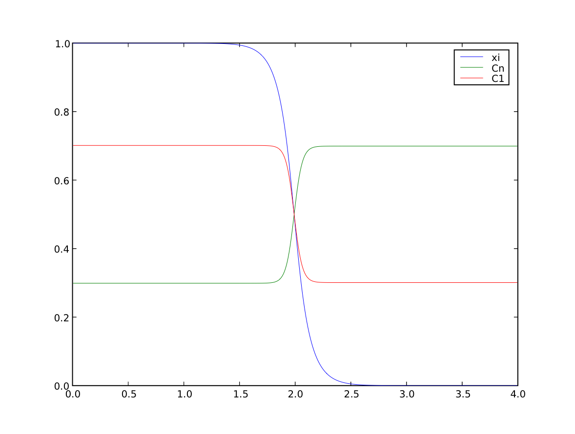
phase and two concentration fields in equilibrium

we confirm that the far-field phases have remained separated

>>> numerix.allclose(phase(((0., L),)), (1.0, 0.0), rtol = 1e-5, atol = 1e-5)
1

and that the solute concentration field has appropriately segregated into solute-rich and solute-poor phases.

>>> print(numerix.allclose(substitutionals[0](((0., L),)), (0.7, 0.3), rtol = 2e-3, atol = 2e-3))
1

The same system of equations can model a quaternary substitutional system as easily as a binary. Because it depends on the number of substitutional solute species in question, we recreate the solvent

>>> solvent = ComponentVariable(mesh = mesh, name = 'Cn', value = 1.)

and make three new solute species

>>> substitutionals = [
...     ComponentVariable(mesh = mesh, name = 'C1',
...                       diffusivity = 1., barrier = 0.,
...                       standardPotential = numerix.log(.3/.4) - numerix.log(.1/.2)),
...     ComponentVariable(mesh = mesh, name = 'C2',
...                       diffusivity = 1., barrier = 0.,
...                       standardPotential = numerix.log(.4/.3) - numerix.log(.1/.2)),
...     ComponentVariable(mesh = mesh, name = 'C3',
...                       diffusivity = 1., barrier = 0.,
...                       standardPotential = numerix.log(.2/.1) - numerix.log(.1/.2))]

>>> for component in substitutionals:
...     solvent -= component
>>> solvent.standardPotential = numerix.log(.1/.2)
>>> solvent.barrier = 1.

These thermodynamic parameters are chosen to give a solid phase rich in the solvent and the first substitutional component and a liquid phase rich in the remaining two substitutional species.

Again, if we’re running interactively, we create a viewer

>>> if __name__ == '__main__':
...     viewer = Viewer(vars=([phase, solvent]
...                           + substitutionals + interstitials),
...                     datamin=0, datamax=1)
...     viewer.plot()

We reinitialize the sharp phase boundary

>>> phase.setValue(1.)
>>> phase.setValue(0., where=x > L / 2)

and the uniform concentration fields, with the substitutional concentrations $C_{1} = C_{2} = 0.35$ and $C_{3} = 0.15$ .

>>> substitutionals[0].setValue(0.35)
>>> substitutionals[1].setValue(0.35)
>>> substitutionals[2].setValue(0.15)

We make new equations

>>> makeEquations(phase, substitutionals, interstitials)

and again iterate to equilibrium

>>> dt = 10000
>>> from builtins import range
>>> for i in range(5):
...     for field in [phase] + substitutionals + interstitials:
...         field.updateOld()
...     phase.equation.solve(var = phase, dt = dt)
...     for field in substitutionals + interstitials:
...         field.equation.solve(var=field,
...                              dt=dt,
...                              solver=field.solver)
...     if __name__ == '__main__':
...         viewer.plot()

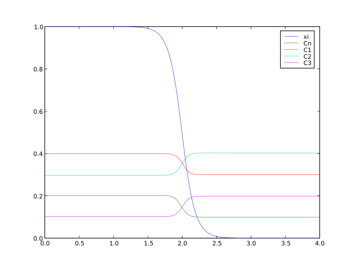
phase and four concentration fields in equilibrium

We confirm that the far-field phases have remained separated

>>> numerix.allclose(phase(((0., L),)), (1.0, 0.0), rtol = 1e-5, atol = 1e-5)
1

and that the concentration fields have appropriately segregated into their respective phases

>>> numerix.allclose(substitutionals[0](((0., L),)), (0.4, 0.3), rtol = 3e-3, atol = 3e-3)
1
>>> numerix.allclose(substitutionals[1](((0., L),)), (0.3, 0.4), rtol = 3e-3, atol = 3e-3)
1
>>> numerix.allclose(substitutionals[2](((0., L),)), (0.1, 0.2), rtol = 3e-3, atol = 3e-3)
1

Finally, we can represent a system that contains both substitutional and interstitial species. We recreate the solvent

>>> solvent = ComponentVariable(mesh = mesh, name = 'Cn', value = 1.)

and two new solute species

>>> substitutionals = [
...     ComponentVariable(mesh = mesh, name = 'C2',
...                       diffusivity = 1., barrier = 0.,
...                       standardPotential = numerix.log(.4/.3) - numerix.log(.4/.6)),
...     ComponentVariable(mesh = mesh, name = 'C3',
...                       diffusivity = 1., barrier = 0.,
...                       standardPotential = numerix.log(.2/.1) - numerix.log(.4/.6))]

and one interstitial

>>> interstitials = [
...     ComponentVariable(mesh = mesh, name = 'C1',
...                       diffusivity = 1., barrier = 0.,
...                       standardPotential = numerix.log(.3/.4) - numerix.log(1.3/1.4))]

>>> for component in substitutionals:
...     solvent -= component
>>> solvent.standardPotential = numerix.log(.4/.6) - numerix.log(1.3/1.4)
>>> solvent.barrier = 1.

These thermodynamic parameters are chosen to give a solid phase rich in interstitials and the solvent and a liquid phase rich in the two substitutional species.

Once again, if we’re running interactively, we create a viewer

>>> if __name__ == '__main__':
...     viewer = Viewer(vars=([phase, solvent]
...                           + substitutionals + interstitials),
...                     datamin=0, datamax=1)
...     viewer.plot()

We reinitialize the sharp phase boundary

>>> phase.setValue(1.)
>>> phase.setValue(0., where=x > L / 2)

and the uniform concentration fields, with the interstitial concentration $C_{1} = 0.35$

>>> interstitials[0].setValue(0.35)

and the substitutional concentrations $C_{2} = 0.35$ and $C_{3} = 0.15$ .

>>> substitutionals[0].setValue(0.35)
>>> substitutionals[1].setValue(0.15)

We make new equations

>>> makeEquations(phase, substitutionals, interstitials)

and again iterate to equilibrium

>>> dt = 10000
>>> from builtins import range
>>> for i in range(5):
...     for field in [phase] + substitutionals + interstitials:
...         field.updateOld()
...     phase.equation.solve(var = phase, dt = dt)
...     for field in substitutionals + interstitials:
...         field.equation.solve(var=field,
...                              dt=dt,
...                              solver=field.solver)
...     if __name__ == '__main__':
...         viewer.plot()

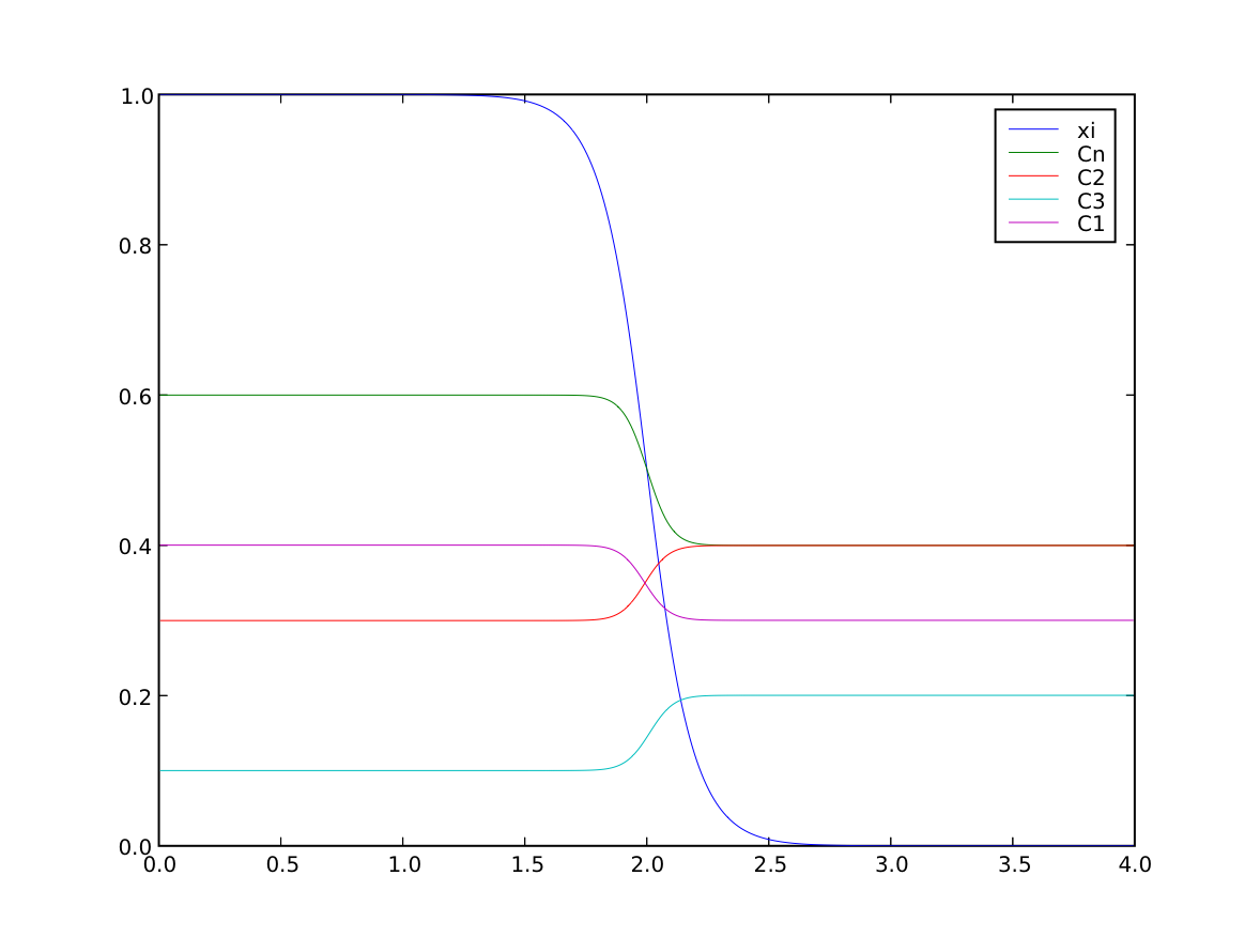
phase and four concentration fields (one like electrons) in equilibrium

We once more confirm that the far-field phases have remained separated

>>> numerix.allclose(phase(((0., L),)), (1.0, 0.0), rtol = 1e-5, atol = 1e-5)
1

and that the concentration fields have appropriately segregated into their respective phases

>>> numerix.allclose(interstitials[0](((0., L),)), (0.4, 0.3), rtol = 3e-3, atol = 3e-3)
1
>>> numerix.allclose(substitutionals[0](((0., L),)), (0.3, 0.4), rtol = 3e-3, atol = 3e-3)
1
>>> numerix.allclose(substitutionals[1](((0., L),)), (0.1, 0.2), rtol = 3e-3, atol = 3e-3)
1

Last updated on Feb 14, 2025. Created using Sphinx 7.1.2.

examples.elphf.phaseDiffusion¶

Versions

Downloads

GitHub