examples.cahnHilliard.mesh3D

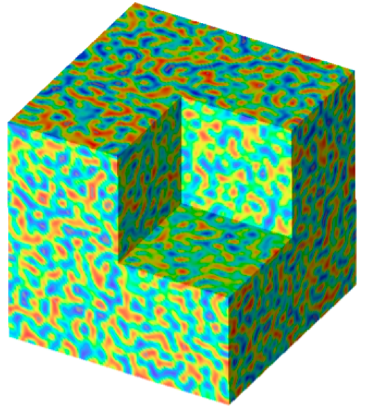
Solves the Cahn-Hilliard problem in a 3D cube

>>> from fipy import CellVariable, Grid3D, Viewer, GaussianNoiseVariable, TransientTerm, DiffusionTerm, DefaultSolver
>>> from fipy.tools import numerix

The only difference from examples.cahnHilliard.mesh2D is the declaration of mesh.

>>> if __name__ == "__main__":
...     nx = ny = nz = 100
... else:
...     nx = ny = nz = 10
>>> mesh = Grid3D(nx=nx, ny=ny, nz=nz, dx=0.25, dy=0.25, dz=0.25)
>>> phi = CellVariable(name=r"$\phi$", mesh=mesh)

We start the problem with random fluctuations about \(\phi = 1/2\)

>>> phi.setValue(GaussianNoiseVariable(mesh=mesh,
...                                    mean=0.5,
...                                    variance=0.01))

FiPy doesn’t plot or output anything unless you tell it to:

>>> if __name__ == "__main__":
...     viewer = Viewer(vars=(phi,), datamin=0., datamax=1.)

For FiPy, we need to perform the partial derivative \(\partial f/\partial \phi\) manually and then put the equation in the canonical form by decomposing the spatial derivatives so that each Term is of a single, even order:

\[\frac{\partial \phi}{\partial t} = \nabla\cdot D a^2 \left[ 1 - 6 \phi \left(1 - \phi\right)\right] \nabla \phi- \nabla\cdot D \nabla \epsilon^2 \nabla^2 \phi.\]

FiPy would automatically interpolate D * a**2 * (1 - 6 * phi * (1 - phi)) onto the faces, where the diffusive flux is calculated, but we obtain somewhat more accurate results by performing a linear interpolation from phi at cell centers to PHI at face centers. Some problems benefit from non-linear interpolations, such as harmonic or geometric means, and FiPy makes it easy to obtain these, too.

>>> PHI = phi.arithmeticFaceValue
>>> D = a = epsilon = 1.
>>> eq = (TransientTerm()
...       == DiffusionTerm(coeff=D * a**2 * (1 - 6 * PHI * (1 - PHI)))
...       - DiffusionTerm(coeff=(D, epsilon**2)))

Because the evolution of a spinodal microstructure slows with time, we use exponentially increasing time steps to keep the simulation “interesting”. The FiPy user always has direct control over the evolution of their problem.

>>> dexp = -5
>>> elapsed = 0.
>>> if __name__ == "__main__":
...     duration = 1000.
... else:
...     duration = 1e-2
>>> while elapsed < duration:
...     dt = min(100, numerix.exp(dexp))
...     elapsed += dt
...     dexp += 0.01
...     eq.solve(phi, dt=dt, solver=DefaultSolver(precon=None))
...     if __name__ == "__main__":
...         viewer.plot()

Last updated on Sep 16, 2025. Created using Sphinx 7.1.2.