A (Relatively) Simple Example
The Uncertainty in a Resistor Network
Let's imaging that we have a resistor network that looks like this:
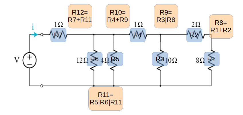
Let's assume that each resistor is known with ± 5% accuracy. What is the effective resistance of the network and the associated uncertainty?
using NeXLUncertaintiesFirst let's define a label to help us uniquely identify the resistors. The integer indices will be those in the blue (input) and peach (intermediate) boxes on the diagram above.
struct Resistor <: Label
    index::Integer
end

Base.show(io::IO, r::Resistor) = print(io, "R$(r.index)")
First, let's design the measurement model for the resistors in series. The resistance is just the sum of the resistors involved and the derivative is unity for these resistors and zero for the other resistors.
struct Series <: MeasurementModel
    resistors::Vector{Resistor}
    outindex::Int
end

Base.show(io::IO, ss::Series) = print(io,"Rmodel[$(ss.outindex)]")

function NeXLUncertainties.compute(ss::Series, inputs::LabeledValues, withJac::Bool=false)
    resistance = sum(inputs[r] for r in ss.resistors)
    vals = LabeledValues( (Resistor(ss.outindex ), ), ( resistance, ) )
    if withJac
        jac= zeros(1, length(inputs))
        for r in ss.resistors
            jac[1, indexin(inputs, r)] = 1.0
        end
    else
        jac = nothing
    end
    return (vals, jac)
end
Then the model for the resistors in parallel. The resistance is the reciprocal of the sum of reciprocals of the resistors involved.
struct Parallel <: MeasurementModel
    resistors::Vector{Resistor}
    outindex::Integer
end

Base.show(io::IO, ss::Series) = print(io,"Rmodel[$(ss.outindex)]")

function NeXLUncertainties.compute(ss::Parallel, inputs::LabeledValues, withJac::Bool=false)
    resistance = 1.0/sum(1.0/inputs[r] for r in ss.resistors)
    vals = LabeledValues( (Resistor(ss.outindex ), ), ( resistance, ) )
    if withJac
        jac = zeros(1, length(inputs))
        for r in ss.resistors
            jac[1, indexin(inputs, r)] = (resistance/inputs[r])^2
        end
    end
    return (vals, jac)
end
We'll define the input resistors' properties.
# Define the inital resistors
resistor = Resistor.(1:7)
resistance = [ 8.0, 2.0, 10.0, 1.0, 4.0, 12.0, 1.0 ]
dresistance = (0.05*resistance).^2
inputs = uvs(resistor,resistance,dresistance)| Labels | Values | R1 | R2 | R3 | R4 | R5 | R6 | R7 | |
|---|---|---|---|---|---|---|---|---|---|
| R1 | 8.00e+00 | (4.00e-01)² | 0.00e+00 | 0.00e+00 | 0.00e+00 | 0.00e+00 | 0.00e+00 | 0.00e+00 | |
| R2 | 2.00e+00 | 0.00e+00 | (1.00e-01)² | 0.00e+00 | 0.00e+00 | 0.00e+00 | 0.00e+00 | 0.00e+00 | |
| R3 | 1.00e+01 | 0.00e+00 | 0.00e+00 | (5.00e-01)² | 0.00e+00 | 0.00e+00 | 0.00e+00 | 0.00e+00 | |
| R4 | 1.00e+00 | ± | 0.00e+00 | 0.00e+00 | 0.00e+00 | (5.00e-02)² | 0.00e+00 | 0.00e+00 | 0.00e+00 |
| R5 | 4.00e+00 | 0.00e+00 | 0.00e+00 | 0.00e+00 | 0.00e+00 | (2.00e-01)² | 0.00e+00 | 0.00e+00 | |
| R6 | 1.20e+01 | 0.00e+00 | 0.00e+00 | 0.00e+00 | 0.00e+00 | 0.00e+00 | (6.00e-01)² | 0.00e+00 | |
| R7 | 1.00e+00 | 0.00e+00 | 0.00e+00 | 0.00e+00 | 0.00e+00 | 0.00e+00 | 0.00e+00 | (5.00e-02)² |
Then we will define a model to descibe each step in the network resistor. In each step, I've defined the model as the Series or Parallel combination of the resistors plus AllInputs() | to pass the input variables from this step onto the next. (Putting AllInputs() up front maintains the ordering of variables.)
r8 = AllInputs() | Series([resistor[1], resistor[2]], 8)
r9 = AllInputs() | Parallel([Resistor(8), resistor[3]], 9)
r10 = AllInputs() | Series([resistor[4], Resistor(9)], 10)
r11 = AllInputs() | Parallel([resistor[5], resistor[6], Resistor(10)], 11)
r12 = AllInputs() | Series([resistor[7], Resistor(11)], 12);
Finally, we pull together the steps into the overall model using the ∘ or compose operator.
model = r12 ∘ r11 ∘ r10 ∘ r9 ∘ r8
res = model(inputs)| Labels | Values | R1 | R2 | R3 | R4 | R5 | R6 | R7 | R8 | R9 | R10 | R11 | R12 | |
|---|---|---|---|---|---|---|---|---|---|---|---|---|---|---|
| R1 | 8.00e+00 | (4.00e-01)² | 0.00e+00 | 0.00e+00 | 0.00e+00 | 0.00e+00 | 0.00e+00 | 0.00e+00 | 1.60e-01 | 4.00e-02 | 4.00e-02 | 4.44e-03 | 4.44e-03 | |
| R2 | 2.00e+00 | 0.00e+00 | (1.00e-01)² | 0.00e+00 | 0.00e+00 | 0.00e+00 | 0.00e+00 | 0.00e+00 | 1.00e-02 | 2.50e-03 | 2.50e-03 | 2.78e-04 | 2.78e-04 | |
| R3 | 1.00e+01 | 0.00e+00 | 0.00e+00 | (5.00e-01)² | 0.00e+00 | 0.00e+00 | 0.00e+00 | 0.00e+00 | 0.00e+00 | 6.25e-02 | 6.25e-02 | 6.94e-03 | 6.94e-03 | |
| R4 | 1.00e+00 | 0.00e+00 | 0.00e+00 | 0.00e+00 | (5.00e-02)² | 0.00e+00 | 0.00e+00 | 0.00e+00 | 0.00e+00 | 0.00e+00 | 2.50e-03 | 2.78e-04 | 2.78e-04 | |
| R5 | 4.00e+00 | 0.00e+00 | 0.00e+00 | 0.00e+00 | 0.00e+00 | (2.00e-01)² | 0.00e+00 | 0.00e+00 | 0.00e+00 | 0.00e+00 | 0.00e+00 | 1.00e-02 | 1.00e-02 | |
| R6 | 1.20e+01 | ± | 0.00e+00 | 0.00e+00 | 0.00e+00 | 0.00e+00 | 0.00e+00 | (6.00e-01)² | 0.00e+00 | 0.00e+00 | 0.00e+00 | 0.00e+00 | 1.00e-02 | 1.00e-02 |
| R7 | 1.00e+00 | 0.00e+00 | 0.00e+00 | 0.00e+00 | 0.00e+00 | 0.00e+00 | 0.00e+00 | (5.00e-02)² | 0.00e+00 | 0.00e+00 | 0.00e+00 | 0.00e+00 | 2.50e-03 | |
| R8 | 1.00e+01 | 1.60e-01 | 1.00e-02 | 0.00e+00 | 0.00e+00 | 0.00e+00 | 0.00e+00 | 0.00e+00 | (4.12e-01)² | 4.25e-02 | 4.25e-02 | 4.72e-03 | 4.72e-03 | |
| R9 | 5.00e+00 | 4.00e-02 | 2.50e-03 | 6.25e-02 | 0.00e+00 | 0.00e+00 | 0.00e+00 | 0.00e+00 | 4.25e-02 | (1.62e-01)² | 2.63e-02 | 2.92e-03 | 2.92e-03 | |
| R10 | 6.00e+00 | 4.00e-02 | 2.50e-03 | 6.25e-02 | 2.50e-03 | 0.00e+00 | 0.00e+00 | 0.00e+00 | 4.25e-02 | 2.63e-02 | (1.70e-01)² | 3.19e-03 | 3.19e-03 | |
| R11 | 2.00e+00 | 4.44e-03 | 2.78e-04 | 6.94e-03 | 2.78e-04 | 1.00e-02 | 1.00e-02 | 0.00e+00 | 4.72e-03 | 2.92e-03 | 3.19e-03 | (5.60e-02)² | 3.13e-03 | |
| R12 | 3.00e+00 | 4.44e-03 | 2.78e-04 | 6.94e-03 | 2.78e-04 | 1.00e-02 | 1.00e-02 | 2.50e-03 | 4.72e-03 | 2.92e-03 | 3.19e-03 | 3.13e-03 | (7.51e-02)² |
To access the single uncertain value associated with the result:
res[Resistor(12)]3.000 ± 0.075You might have noticed that this example is actually a univariate measurement model. There is a simpler way to handle this model using the Measurements package.
First let's define our model equations and check that they produce the same number as above.
pp(a,b) = 1.0/(1.0/a+1.0/b)
pp(a,b,c) = 1.0/(1.0/a+1.0/b+1.0/c)
ss(a,b) = a + b

ss(1.0,pp(12.0,4.0,ss(1.0,pp(10.0,ss(2.0,8.0)))))3.0Yes, they do. Now let's use Measurements to perform the same calculation. We'll define the resistances with uncertainties using Measurements simplified syntax and then we will use the same functions we just used above to compute the model using the values with uncertainties.
using Measurements

r1 = 8.0 ± 0.4
r2 = 2.0 ± 0.1
r3 = 10.0 ± 0.5
r4 = 1.0 ± 0.05
r5 = 4.0 ± 0.2
r6 = 12.0 ± 0.6
r7 = 1.0 ± 0.05

ss(r7,pp(r6,r5,ss(r4,pp(r3,ss(r2,r1)))))
3.0 ± 0.075We do, in fact, get the same result. Take away - For univariate measurement models Measurements is easier. For multivariate measurement models, NeXLUncertainies is necessary.