Applying Analytical Correction to hardness of collisions for HTP
Provided in the MATS v2 release are several examples highlighting MATS capabilities, which can be found in the MATS examples folder.
Dicke narrowing accounts for effective narrowing of the doppler width because of velocity changing collisions. The magnitude of this effect is dependent on the hardness of the collisions. Different line shapes make different assumptions on the hardness of the collision with the Nelkhin-Ghatak making the assumption that collisions are hard, meaning that the molecular velocity before a collision is forgotten after the collision, and the Galatry profile assuming collisions are soft, meaning that many collisions are necessary to change the velocity. In reality, the hardness of the collision is related to the perturbers and absorbers being studied and acts on a continuum. In a paper by Konefał et al. (citation below), authors map the hard Dicke Narrowing term onto the billiard ball collision model, based on a parameter beta, which is related to the pressure (parameterized as the Dicke narrowing at a pressure relative to the doppler width) and the ratio of the masses between the perturber and absorber. As Beta can be calculated, this correction provides a more robust modeling of the Dicke Narrowing without the addition of additional floated parameters.
Simulate Spectrum Objects
Module import follows from the Fitting Experimental Spectra and Fitting Synthetic Spectra examples with additional details on how to simulate spectra found in Fitting Synthetic Spectra and the source documentation.
After the generic parameters are introduced the line list for simulations is read in using the LoadLineListData() function. In this example we are making some adjustments to the line list before simulating. In the MATS fitting, simulations are only conducted to some user-defined range outside of the spectral frequency range (wave_range = 1.5 \(cm^{-1}\) in the current example). This same constraint is not imposed when simulating spectra. This can lead to some far-wing issues between simulation and fitting if care is not taken to match the wave_range to the lines in the parameter linelist and the simulation wing_cutoff magnitude, which should also match the fit wing_cutoff magnitude. For this example, we are truncating the simulation line list to [wave_min - wave_range, wave_max + wave_range]. Additionally, values for the Dicke Narrowing air and self parameters are set and the line mixing terms are set to 0.
from MATS.linelistdata import linelistdata
from MATS import simulate_spectrum

#Generic Fit Parameters
wave_range = 1.5 #range outside of experimental x-range to simulate
IntensityThreshold = 1e-30 #intensities must be above this value to be simulated
Fit_Intensity = 1e-25 #intensities must be above this value for the line to be fit
order_baseline_fit = 1
wave_min = 6326 #cm-1
wave_max = 6328 #cm-1
wave_space = 0.005 #cm-1
baseline_terms = [0] #polynomial baseline coefficients where the index is equal to the coefficient order
etalon = {}

#Read in  linelists
PARAM_LINELIST = linelistdata['CO2_30012']
##Adjust the linelist before simualting spectra
PARAM_LINELIST = pd.read_csv('CO2_30012.csv')
PARAM_LINELIST = PARAM_LINELIST[(PARAM_LINELIST['nu']>= wave_min - wave_range) & (PARAM_LINELIST['nu']<= wave_min + wave_range)]
PARAM_LINELIST.loc[(PARAM_LINELIST['sw'] > Fit_Intensity)& (PARAM_LINELIST['local_iso_id'] == 1) & (PARAM_LINELIST['molec_id'] == 2), 'nuVC_air'] = 0.018596
PARAM_LINELIST.loc[(PARAM_LINELIST['sw'] > Fit_Intensity) & (PARAM_LINELIST['local_iso_id'] == 1) & (PARAM_LINELIST['molec_id'] == 2), 'nuVC_self'] = 0.01993
PARAM_LINELIST.loc[(PARAM_LINELIST['sw'] > Fit_Intensity) & (PARAM_LINELIST['local_iso_id'] == 1) & (PARAM_LINELIST['molec_id'] == 2), 'y_self_296'] = 0
PARAM_LINELIST.loc[(PARAM_LINELIST['sw'] > Fit_Intensity) & (PARAM_LINELIST['local_iso_id'] == 1) & (PARAM_LINELIST['molec_id'] == 2), 'y_air_296'] = 0
For the purpose of showing the mechanism, we will be simulating data for \(CO_{2}\), air, and 10% \(CO_{2}\) in air samples between 1 and 500 torr. The structure of the script follows that outlined in the Fitting Synthetic Spectra example.
The simulate_spectrum() function is used to generate several spectrum class objects. The beta_formalism variable is set to True, which simulates the spectra accounting for the change in Dicke Narrowing with the hardness of the collision. The synthetic spectra span 3 samples: \(CO_{2}\), air, and 10% \(CO_{2}\) in air. The air and \(CO_{2}\) samples can use the diluent = ‘air’ and ‘self’ variables as the Diluent variable can be auto-generated. However, the 10% \(CO_{2}\) in air sample requires the explicit definition of the Diluent variable, which is a dictionary of dictionaries where each diluent is a dictionary with composition and mass (m) keys. This allows the calculation of the mass of perturber, which is necessary for the \(\beta\) implementation. The use of the self term will generate a warning to consider switching to an explicitly name the broadener. This warning is to have the user consider if this is causing ambiguity or unanticipated behavior. Specifically, this could be an issue in multi-species fits or if the explict broadener and self term are both used. To remove the use of the self broadening, have the line shape parameter file with the explicit broadener (ie. gamma0_CO2 instead of gamma0_self) and use the Diluent sample definition as modeled for the 10% \(CO_{2}\) in air sample (ie pure \(CO_{2}\) would be Diluent = {‘CO2’:{‘composition’:1, ‘m’:43.98983} }).
#Synthetic Air Simulation
print ('Synthetic Air Samples')
spec_1 =  simulate_spectrum(PARAM_LINELIST, wave_min, wave_max, wave_space, wave_error = wave_error,
                     SNR = SNR, baseline_terms = baseline_terms, temperature = 25, pressure = 1, diluent = 'air',filename = 'Air_1_torr',
                     wing_cutoff = 25, wing_method = 'wing_wavenumbers',  molefraction = {2 :400*1e-6},
                     etalons = etalon, natural_abundance = True, nominal_temperature = 296, IntensityThreshold = 1e-30, num_segments = 1, beta_formalism = True)
spec_2 =  simulate_spectrum(PARAM_LINELIST, wave_min, wave_max, wave_space, wave_error = wave_error,
                     SNR = SNR, baseline_terms = baseline_terms, temperature = 25, pressure = 10, diluent = 'air',filename = 'Air_10_torr',
                     wing_cutoff = 25, wing_method = 'wing_wavenumbers',  molefraction = {2 :400*1e-6},
                     etalons = etalon, natural_abundance = True, nominal_temperature = 296, IntensityThreshold = 1e-30, num_segments = 1, beta_formalism = True)
spec_3 =  simulate_spectrum(PARAM_LINELIST, wave_min, wave_max, wave_space, wave_error = wave_error,
                     SNR = SNR, baseline_terms = baseline_terms, temperature = 25, pressure = 100, diluent = 'air',filename = 'Air_100_torr',
                     wing_cutoff = 25, wing_method = 'wing_wavenumbers', molefraction = {2 :400*1e-6},
                     etalons = etalon, natural_abundance = True, nominal_temperature = 296, IntensityThreshold = 1e-30, num_segments = 1, beta_formalism = True)
spec_4 =  simulate_spectrum(PARAM_LINELIST, wave_min, wave_max, wave_space, wave_error = wave_error,
                     SNR = SNR, baseline_terms = baseline_terms, temperature = 25, pressure = 250, diluent = 'air',filename = 'Air_250_torr',
                     wing_cutoff = 25, wing_method = 'wing_wavenumbers', molefraction = {2 :400*1e-6},
                     etalons = etalon, natural_abundance = True, nominal_temperature = 296, IntensityThreshold = 1e-30, num_segments = 1, beta_formalism = True)
spec_5 =  simulate_spectrum(PARAM_LINELIST, wave_min, wave_max, wave_space, wave_error = wave_error,
                     SNR = SNR, baseline_terms = baseline_terms, temperature = 25, pressure = 500, diluent = 'air',filename = 'Air_500_torr',
                    wing_cutoff = 25, wing_method = 'wing_wavenumbers',  molefraction = {2 :400*1e-6},
                     etalons = etalon, natural_abundance = True, nominal_temperature = 296, IntensityThreshold = 1e-30, num_segments = 1, beta_formalism = True)
#Mixture of CO2 and Air
## Note that we had to use the Diluent method opposedc to the diluent method.  Additionally, the use of the self broadening term will generate some warnings
print ('Mixture Samples')
spec_6 =  simulate_spectrum(PARAM_LINELIST, wave_min, wave_max, wave_space, wave_error = wave_error,
                     SNR = SNR, baseline_terms = baseline_terms, temperature = 25, pressure = 1, filename = 'Mix_1_torr',
                     Diluent = {'self':{'composition':0.1, 'm':43.98983} , 'air' :{'composition':0.9, 'm':28.95734}},
                     wing_cutoff = 25, wing_method = 'wing_wavenumbers',  molefraction = {2 :0.1},
                     etalons = etalon, natural_abundance = True, nominal_temperature = 296, IntensityThreshold = 1e-30, num_segments = 1, beta_formalism = True)
spec_7=  simulate_spectrum(PARAM_LINELIST, wave_min, wave_max, wave_space, wave_error = wave_error,
                     SNR = SNR, baseline_terms = baseline_terms, temperature = 25, pressure = 10, filename = 'Mix_10_torr',
                     Diluent = {'self':{'composition':0.1, 'm':43.98983} , 'air' :{'composition':0.9, 'm':28.95734}},
                     wing_cutoff = 25, wing_method = 'wing_wavenumbers',  molefraction = {2 :0.1},
                     etalons = etalon, natural_abundance = True, nominal_temperature = 296, IntensityThreshold = 1e-30, num_segments = 1, beta_formalism = True)
spec_8 =  simulate_spectrum(PARAM_LINELIST, wave_min, wave_max, wave_space, wave_error = wave_error,
                     SNR = SNR, baseline_terms = baseline_terms, temperature = 25, pressure = 100, filename = 'Mix_100_torr',
                     Diluent = {'self':{'composition':0.1, 'm':43.98983} , 'air' :{'composition':0.9, 'm':28.95734}},
                     wing_cutoff = 25, wing_method = 'wing_wavenumbers',  molefraction = {2 :0.1},
                     etalons = etalon, natural_abundance = True, nominal_temperature = 296, IntensityThreshold = 1e-30, num_segments = 1, beta_formalism = True)
spec_9 =  simulate_spectrum(PARAM_LINELIST, wave_min, wave_max, wave_space, wave_error = wave_error,
                     SNR = SNR, baseline_terms = baseline_terms, temperature = 25, pressure = 250,filename = 'Mix_250_torr',
                     Diluent = {'self':{'composition':0.1, 'm':43.98983} , 'air' :{'composition':0.9, 'm':28.95734}},
                     wing_cutoff = 25, wing_method = 'wing_wavenumbers', molefraction = {2 :0.1},
                     etalons = etalon, natural_abundance = True, nominal_temperature = 296, IntensityThreshold = 1e-30, num_segments = 1, beta_formalism = True)
spec_10 =  simulate_spectrum(PARAM_LINELIST, wave_min, wave_max, wave_space, wave_error = wave_error,
                     SNR = SNR, baseline_terms = baseline_terms, temperature = 25, pressure = 500, filename = 'Mix_500_torr',
                          Diluent = {'self':{'composition':0.1, 'm':43.98983} , 'air' :{'composition':0.9, 'm':28.95734}},
                     wing_cutoff = 25, wing_method = 'wing_wavenumbers', molefraction = {2 :0.1},
                     etalons = etalon, natural_abundance = True, nominal_temperature = 296, IntensityThreshold = 1e-30, num_segments = 1, beta_formalism = True)

#Pure CO2.  Notice that the use of the self broadening term will cause some warnings.
print ('Pure CO2 Samples')
spec_11 =  simulate_spectrum(PARAM_LINELIST, wave_min, wave_max, wave_space, wave_error = wave_error,
                     SNR = SNR, baseline_terms = baseline_terms, temperature = 25, pressure = 1, diluent = 'self', filename = 'CO2_1_torr',
                     wing_cutoff = 25, wing_method = 'wing_wavenumbers',  molefraction = {2 :1},
                     etalons = etalon, natural_abundance = True, nominal_temperature = 296, IntensityThreshold = 1e-30, num_segments = 1, beta_formalism = True)
spec_12 =  simulate_spectrum(PARAM_LINELIST, wave_min, wave_max, wave_space, wave_error = wave_error,
                     SNR = SNR, baseline_terms = baseline_terms, temperature = 25, pressure = 10, diluent = 'self',filename = 'CO2_10_torr',
                     wing_cutoff = 25, wing_method = 'wing_wavenumbers',  molefraction = {2 :1},
                     etalons = etalon, natural_abundance = True, nominal_temperature = 296, IntensityThreshold = 1e-30, num_segments = 1, beta_formalism = True)
spec_13 =  simulate_spectrum(PARAM_LINELIST, wave_min, wave_max, wave_space, wave_error = wave_error,
                     SNR = SNR, baseline_terms = baseline_terms, temperature = 25, pressure = 100, diluent = 'self',filename = 'CO2_100_torr',
                     wing_cutoff = 25, wing_method = 'wing_wavenumbers',  molefraction = {2 :1},
                     etalons = etalon, natural_abundance = True, nominal_temperature = 296, IntensityThreshold = 1e-30, num_segments = 1, beta_formalism = True)
spec_14 =  simulate_spectrum(PARAM_LINELIST, wave_min, wave_max, wave_space, wave_error = wave_error,
                     SNR = SNR, baseline_terms = baseline_terms, temperature = 25, pressure = 250,  diluent = 'self', filename = 'CO2_250_torr',
                     wing_cutoff = 25, wing_method = 'wing_wavenumbers', molefraction = {2 :1},
                     etalons = etalon, natural_abundance = True, nominal_temperature = 296, IntensityThreshold = 1e-30, num_segments = 1, beta_formalism = True)
spec_15 =  simulate_spectrum(PARAM_LINELIST, wave_min, wave_max, wave_space, wave_error = wave_error,
                     SNR = SNR, baseline_terms = baseline_terms, temperature = 25, pressure = 500,  diluent = 'self', filename = 'CO2_500_torr',
                     wing_cutoff = 25, wing_method = 'wing_wavenumbers', molefraction = {2 :1},
                     etalons = etalon, natural_abundance = True, nominal_temperature = 296, IntensityThreshold = 1e-30, num_segments = 1, beta_formalism = True)
Generate Dataset and Fit Parameter Files
Following the procedure outlined in Fitting Synthetic Spectra and Fitting Experimental Spectra. This example is using the SDNGP without line mixing, is constraining all parameters to multi-spectrum fits, and is floating the line center, line intensity, collisional broadening, pressure shift, speed-dependent broadening, and Dicke narrowing terms.
SPECTRA = MATS.Dataset([spec_1, spec_2, spec_3, spec_4, spec_5, spec_6, spec_7, spec_8, spec_9, spec_10, spec_11, spec_12, spec_13, spec_14, spec_15], 'CO2 Study',PARAM_LINELIST )

#Generate Baseline Parameter list based on number of etalons in spectra definitions and baseline order
BASE_LINELIST = SPECTRA.generate_baseline_paramlist()
FITPARAMS = MATS.Generate_FitParam_File(SPECTRA, PARAM_LINELIST, BASE_LINELIST, lineprofile = 'SDNGP', linemixing = False,
                               fit_intensity = Fit_Intensity, threshold_intensity = IntensityThreshold, sim_window = wave_range,
                               nu_constrain = True, sw_constrain = True, gamma0_constrain = True, delta0_constrain = True,
                                aw_constrain = True, as_constrain = True,
                                nuVC_constrain = True, eta_constrain =True, linemixing_constrain = True)
                               #additional_columns = ['trans_id', 'local_lower_quanta', 'm'])

FITPARAMS.generate_fit_param_linelist_from_linelist(vary_nu = {2:{1:True, 2:False, 3:False}}, vary_sw = {2:{1:True, 2:False, 3:False}},
                                                 vary_gamma0 = {2:{1: True, 2:False, 3: False}, 1:{1:False}}, vary_n_gamma0 = {2:{1:False}},
                                                 vary_delta0 = {2:{1: True, 2:False, 3: False}, 1:{1:False}}, vary_n_delta0 = {2:{1:False}},
                                                 vary_aw = {2:{1: True, 2:False, 3: False}, 1:{1:False}}, vary_n_gamma2 = {2:{1:False}},
                                                 vary_as = {}, vary_n_delta2 = {2:{1:False}},
                                                 vary_nuVC = {2:{1:True}}, vary_n_nuVC = {2:{1:False}},
                                                 vary_eta = {}, vary_linemixing = {2:{1:False}})

FITPARAMS.generate_fit_baseline_linelist(vary_baseline = False, vary_molefraction = {7:False, 1:Fa   lse}, vary_xshift = False,
                                   vary_etalon_amp= False, vary_etalon_period= False, vary_etalon_phase= False)
Fit Data
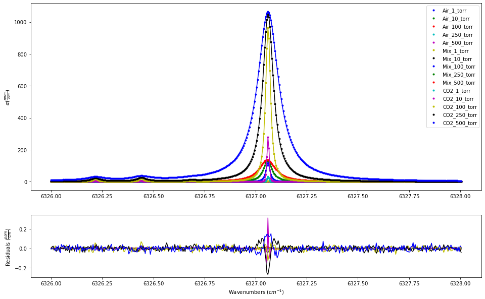
In this first iteration, we are fitting the data without including the beta_formalism to correct for the hardness of the collisions by setting the beta_formalism to False in the Fit_DataSet instance, which is the default. The results show systematic residuals at the line core based on the large range of pressures.
fit_data = MATS.Fit_DataSet(SPECTRA,'Baseline_LineList', 'Parameter_LineList', minimum_parameter_fit_intensity = 1e-24,
                   beta_formalism = False)
params = fit_data.generate_params()
result = fit_data.fit_data(params, wing_cutoff = 25,wing_method = 'wing_wavenumbers')
#print (result.params.pretty_print())

fit_data.residual_analysis(result, indv_resid_plot=False)
fit_data.update_params(result, param_linelist_update_file = 'Results without Beta')
SPECTRA.generate_summary_file(save_file = True)
SPECTRA.plot_model_residuals()
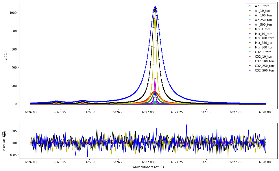
In the second iteration, the beta_formalism term is set to True. Unsuprisingly, using the beta correction gives better results as this is how the spectra were simulated.
fit_data = MATS.Fit_DataSet(SPECTRA,'Baseline_LineList', 'Parameter_LineList', minimum_parameter_fit_intensity = 1e-24,
                   beta_formalism = True)
params = fit_data.generate_params()
result = fit_data.fit_data(params, wing_cutoff = 25,wing_method = 'wing_wavenumbers')
#print (result.params.pretty_print())

fit_data.residual_analysis(result, indv_resid_plot=False)
fit_data.update_params(result)
SPECTRA.generate_summary_file(save_file = True)
SPECTRA.plot_model_residuals()
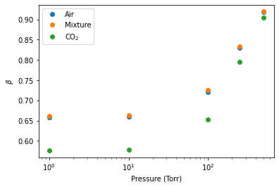
The Fit_DataSet.generate_beta_output_file() definition can be used to tabulate a value of the math:beta parameters that are used for all lines and each spectrum. By default this is saved in a file called Beta Summary File.csv. This plot shows how this math:beta parameter changes with sample and pressure.
fit_data.generate_beta_output_file()
beta_summary_file = pd.read_csv('Beta Summary File.csv', index_col = 0)
beta_summary_file[beta_summary_file['nuVC_air_vary']==True]

pressures = [1,10, 100, 250, 500]
air_beta = [beta_summary_file[beta_summary_file.index == 62]['Beta_1'].values[0], beta_summary_file[beta_summary_file.index == 62]['Beta_2'].values[0], beta_summary_file[beta_summary_file.index == 62]['Beta_3'].values[0],
         beta_summary_file[beta_summary_file.index == 62]['Beta_4'].values[0], beta_summary_file[beta_summary_file.index == 62]['Beta_5'].values[0]]
mix_beta = [beta_summary_file[beta_summary_file.index == 62]['Beta_6'].values[0], beta_summary_file[beta_summary_file.index == 62]['Beta_7'].values[0], beta_summary_file[beta_summary_file.index == 62]['Beta_8'].values[0],
         beta_summary_file[beta_summary_file.index == 62]['Beta_9'].values[0], beta_summary_file[beta_summary_file.index == 62]['Beta_10'].values[0]]
CO2_beta = [beta_summary_file[beta_summary_file.index == 62]['Beta_11'].values[0], beta_summary_file[beta_summary_file.index == 62]['Beta_12'].values, beta_summary_file[beta_summary_file.index == 62]['Beta_13'].values[0],
         beta_summary_file[beta_summary_file.index == 62]['Beta_14'].values[0], beta_summary_file[beta_summary_file.index == 62]['Beta_15'].values[0]]

plt.semilogx(pressures, air_beta, 'o', label = 'Air')
plt.semilogx(pressures, mix_beta, 'o', label = 'Mixture')
plt.semilogx(pressures, CO2_beta, 'o', label = 'CO$_{2}$')
plt.xlabel('Pressure (Torr)')
plt.ylabel('$\\beta$')
plt.legend()
plt.show()