Manifold Active Learning of a Protein Formulation Phase Map

This case study runs a single active learning campaign on the AFL-agent virtual protein / glycerol / temperature instrument, ProteinGlycerolTemperaturePhaseMap, with the manifold strategy of the AFL-bioformulations study. The classifier and the benchmark are the same as in the companion notebook, Grid-Based Active Learning of a Protein Formulation Phase Map; the two grid searches of the acquisition are replaced by continuous optimisations.

1. Classifier. A DirichletGPExtrapolator is fit to the measured phase labels on the three-dimensional design space (protein, temperature, glycerol).

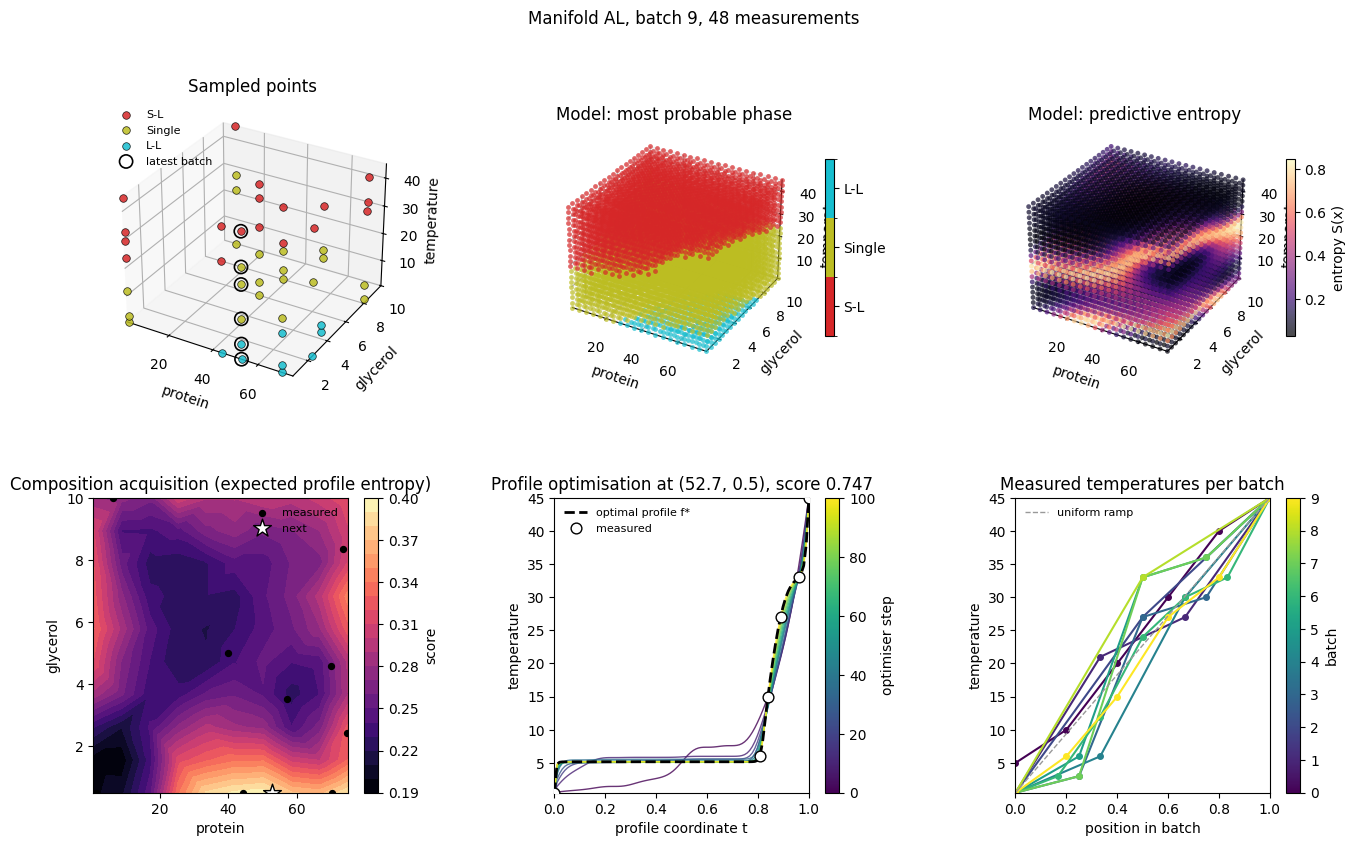
2. Composition. BoTorchAcquisition searches the (protein, glycerol) plane for the composition with the largest expected classifier entropy over random temperature profiles.

3. Temperature profile. At that composition SRSFHilbertSphereAcquisitionFunction optimises a temperature profile (a function on [0, 1] mapped onto the temperature range) on the square-root slope function (SRSF) Hilbert sphere, so that the whole sweep of temperatures passes through the most uncertain regions of the phase map. The optimal profile is discretised into the temperatures that are measured.

The two acquisition scores are plain Python functions defined in this notebook. They take the fitted classifier through a Variable placeholder that the acquisition ops resolve against the dataset at run time.

Set Up the Environment

Import the libraries used in the campaign. The design-space limits, the classifier and acquisition settings, the simulator, the acquisition scores and the pipeline are defined in helpers.py in this folder, which the companion notebook Closed-Loop Manifold Active Learning with AFL Servers shares with the agent server; the plotting functions are in visuals.py. The design-space limits are those of the virtual instrument, standardize=True keeps the feature scaling inside the classifier so all values below are in instrument units.

# Uncomment this cell if you need to install AFL-agent with the ``manifold`` extra
# (torch, gpytorch, pyro-ppl, botorch, geoopt, alphashape, trimesh).
# !pip install "AFL-agent[manifold] @ git+https://github.com/usnistgov/afl-agent"

import matplotlib.pyplot as plt
import numpy as np
import pandas as pd
import torch
import xarray as xr

import helpers  # settings, scores and pipeline, see helpers.py in this folder
from helpers import BOUNDS_T, COMPONENTS, GRID_STEPS, LIMITS, PROFILE, SEED, XY, get_temperature_profile, pipeline, sim
from visuals import plot_manifold_iteration, plot_phase_map, plot_score_history  # plotting, see visuals.py in this folder

np.set_printoptions(precision=3, suppress=True)

/home/knv2/codebase/AFL-bioformulations/.venv/lib/python3.11/site-packages/torch/cuda/__init__.py:182: UserWarning: CUDA initialization: The NVIDIA driver on your system is too old (found version 11040). Please update your GPU driver by downloading and installing a new version from the URL: http://www.nvidia.com/Download/index.aspx Alternatively, go to: https://pytorch.org to install a PyTorch version that has been compiled with your version of the CUDA driver. (Triggered internally at /pytorch/c10/cuda/CUDAFunctions.cpp:119.)
  return torch._C._cuda_getDeviceCount() > 0

# campaign
N_SAMPLES = 10  # number of compositions (one temperature profile each) to acquire
INITIAL_COMPOSITION = {"protein": 40.0, "glycerol": 5.0}  # the one composition measured before the campaign
INITIAL_TEMPERATURES = [5.0, 10.0, 20.0, 30.0, 40.0, 45.0]  # ... and the temperatures it is measured at
PLOT_EVERY_ITERATION = False  # draw the six-panel figure after every iteration (slower, more output)

# everything else comes from helpers.py: SEED (numpy / torch seed and the seed of the benchmark test
# set), LIMITS and BOUNDS_T of the design space, GRID_STEPS, the GP, optimiser and benchmark settings
# and PROFILE, the sampling of the optimal temperature profile
{k: getattr(helpers, k) for k in ["SEED", "LIMITS", "GRID_STEPS", "GP_PARAMS", "OPTIMIZE_XY", "OPTIMIZE_F", "N_MC_PROFILES", "PROFILE", "N_TEST_PER_PHASE", "F1_AVERAGE"]}

{'SEED': 1000,
 'LIMITS': {'protein': (0.5, 75.0),
  'glycerol': (0.5, 10.0),
  'temperature': (0.5, 45.0)},
 'GRID_STEPS': 20,
 'GP_PARAMS': {'method': 'mll', 'n_iterations': 200, 'verbose': False},
 'OPTIMIZE_XY': {'num_restarts': 8, 'raw_samples': 64},
 'OPTIMIZE_F': {'n_restarts': 8, 'n_iterations': 100},
 'N_MC_PROFILES': 16,
 'PROFILE': {'dt': 0.05, 'dT': 3.0},
 'N_TEST_PER_PHASE': 100,
 'F1_AVERAGE': 'weighted'}

The Virtual Instrument

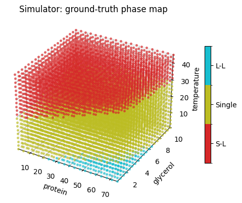
sim is the ProteinGlycerolTemperaturePhaseMap instance created in helpers.py; its measure exposes one (protein, glycerol) composition at several temperatures and returns one sample per temperature with the simulated scattering, the design_space coordinates in the instrument’s feature order and the integer phase label in phases. The feature order of the instrument is what the pipeline and the scores below work in.

# sim, COMPONENTS (feature order of the instrument: protein, temperature, glycerol) and
# XY (composition components: protein, glycerol) are imported from helpers.py
sim.status(), COMPONENTS, XY

(['Idle', 'Configurations Loaded=3', 'Phases Traced=3', 'Noise Level=0.0'],
 ['protein', 'temperature', 'glycerol'],
 ['protein', 'glycerol'])

from AFL.double_agent.benchmarking import virtual_instrument_labels

grid_axes = [np.linspace(*LIMITS[c], GRID_STEPS) for c in COMPONENTS]
grid = np.stack(np.meshgrid(*grid_axes, indexing="ij"), axis=-1).reshape(-1, len(COMPONENTS))
true_labels = virtual_instrument_labels(sim, grid)

plot_phase_map(grid, true_labels, LIMITS, COMPONENTS)
plt.show()

The Acquisition Scores

Both scores reduce to the same quantity: the classifier entropy along temperature profiles at a composition.

A profile is a point q on the SRSF Hilbert sphere; manifold.srsf_to_function(q) turns it back into a function on [0, 1] whose values are mapped onto the temperature range. The design points are assembled in the instrument’s feature order and passed to model.predict.

• composition_score is the BoTorchAcquisition objective: the mean entropy over N_MC_PROFILES random profiles. The same profiles are drawn on every call so the score is a smooth function of the composition for the gradient-based optimiser.

• profile_score is the SRSFHilbertSphereAcquisitionFunction objective: the mean entropy along each candidate profile at the chosen composition. power=1 is the plain mean; larger values favour profiles with a few very uncertain points.

• get_temperature_profile discretises the optimal profile into the unique, rounded temperatures that are measured.

phase_model and composition_next are Variable placeholders. The ops resolve them against the dataset while they calculate: the model reference written by the extrapolator loads into the fitted classifier and the composition chosen in stage 1 becomes a tensor.

The Pipeline

pipeline is defined in helpers.py and is fixed for the whole campaign; only the dataset it is applied to grows:

• CartesianGrid builds the evaluation grids, the DirichletGPExtrapolator fits the classifier and writes its predictions (phase_mean, phase_y_prob, phase_entropy) on the grid and a reference to the fitted model to phase_model, which PhaseMapF1Score loads to score it against the simulator.

• BoTorchAcquisition maximises composition_score over the (protein, glycerol) bounds and reports the score on the composition grid (composition_decision_surface).

• SRSFHilbertSphereAcquisitionFunction runs Riemannian Adam from several random profiles and writes the best profile to profile_function, the optimiser path of the winning restart to profile_trajectory and the loss of every restart to profile_loss.

for i, op in enumerate(pipeline):
    print(i, op.name)

0 Grid-DesignSpace
1 Grid-Composition
2 DirichletGPExtrapolator-PhaseLabels
3 PhaseMapF1Score
4 BoTorchAcquisition-Composition
5 SRSF-TemperatureProfile

Make the Initial Measurement

The campaign starts from a single composition measured at six temperatures. The batch_sample_id variable records which batch a sample came from; it is used to ring the latest batch in the plots.

np.random.seed(SEED)
torch.manual_seed(SEED)

ds_running = sim.measure(
    protein=INITIAL_COMPOSITION["protein"],
    glycerol=INITIAL_COMPOSITION["glycerol"],
    temperatures=INITIAL_TEMPERATURES,
    batch_id=0,
)
temperature_history = {0: np.asarray(INITIAL_TEMPERATURES, dtype=float)}  # batch_id -> measured temperatures
ds_running

<xarray.Dataset> Size: 43kB
Dimensions:          (sample: 6, ds_dim: 3, q: 281, component: 2)
Coordinates:
  * ds_dim           (ds_dim) <U11 132B 'protein' 'temperature' 'glycerol'
  * q                (q) float64 2kB 0.003836 0.004348 ... 0.6293 0.6334
  * component        (component) <U11 88B 'protein' 'glycerol'
Dimensions without coordinates: sample
Data variables:
    design_space     (sample, ds_dim) float64 144B 40.0 5.0 5.0 ... 45.0 5.0
    I                (sample, q) float64 13kB 6.234 6.234 6.233 ... 1.0 1.0 1.0
    I_noiseless      (sample, q) float64 13kB 6.234 6.234 6.233 ... 1.0 1.0 1.0
    dI               (sample, q) float64 13kB 0.0 0.0 0.0 0.0 ... 0.0 0.0 0.0
    phases           (sample) int64 48B 1 1 1 0 0 0
    in_hull          (sample) bool 6B True True True True True True
    composition      (sample, component) float64 96B 40.0 5.0 40.0 ... 40.0 5.0
    batch_sample_id  (sample) int64 48B 0 0 0 0 0 0
Attributes:
    components:      ['protein', 'glycerol']
    components_dim:  component
    labels:          phases

xarray.Dataset

• Dimensions:
  • sample: 6
  • ds_dim: 3
  • q: 281
  • component: 2
• Coordinates: (3)
  • ds_dim
    (ds_dim)
    <U11
    'protein' 'temperature' 'glycerol'

    array(['protein', 'temperature', 'glycerol'], dtype='<U11')

  • q
    (q)
    float64
    0.003836 0.004348 ... 0.6293 0.6334

    array([0.003836, 0.004348, 0.004859, ..., 0.6252  , 0.6293  , 0.6334  ],
          shape=(281,))

  • component
    (component)
    <U11
    'protein' 'glycerol'

    array(['protein', 'glycerol'], dtype='<U11')

• Data variables: (8)
  • design_space
    (sample, ds_dim)
    float64
    40.0 5.0 5.0 40.0 ... 40.0 45.0 5.0

    array([[40.,  5.,  5.],
           [40., 10.,  5.],
           [40., 20.,  5.],
           [40., 30.,  5.],
           [40., 40.,  5.],
           [40., 45.,  5.]])

  • I
    (sample, q)
    float64
    6.234 6.234 6.233 ... 1.0 1.0 1.0

    array([[   6.234,    6.234,    6.233, ...,    1.029,    1.028,    1.027],
           [   6.234,    6.234,    6.233, ...,    1.029,    1.028,    1.027],
           [   6.234,    6.234,    6.233, ...,    1.029,    1.028,    1.027],
           [1326.219,  578.773,  309.578, ...,    1.   ,    1.   ,    1.   ],
           [1326.219,  578.773,  309.578, ...,    1.   ,    1.   ,    1.   ],
           [1326.219,  578.773,  309.578, ...,    1.   ,    1.   ,    1.   ]],
          shape=(6, 281))

  • I_noiseless
    (sample, q)
    float64
    6.234 6.234 6.233 ... 1.0 1.0 1.0

    array([[   6.234,    6.234,    6.233, ...,    1.029,    1.028,    1.027],
           [   6.234,    6.234,    6.233, ...,    1.029,    1.028,    1.027],
           [   6.234,    6.234,    6.233, ...,    1.029,    1.028,    1.027],
           [1326.219,  578.773,  309.578, ...,    1.   ,    1.   ,    1.   ],
           [1326.219,  578.773,  309.578, ...,    1.   ,    1.   ,    1.   ],
           [1326.219,  578.773,  309.578, ...,    1.   ,    1.   ,    1.   ]],
          shape=(6, 281))

  • dI
    (sample, q)
    float64
    0.0 0.0 0.0 0.0 ... 0.0 0.0 0.0 0.0

    array([[0., 0., 0., ..., 0., 0., 0.],
           [0., 0., 0., ..., 0., 0., 0.],
           [0., 0., 0., ..., 0., 0., 0.],
           [0., 0., 0., ..., 0., 0., 0.],
           [0., 0., 0., ..., 0., 0., 0.],
           [0., 0., 0., ..., 0., 0., 0.]], shape=(6, 281))

  • phases
    (sample)
    int64
    1 1 1 0 0 0

    array([1, 1, 1, 0, 0, 0])

  • in_hull
    (sample)
    bool
    True True True True True True

    array([ True,  True,  True,  True,  True,  True])

  • composition
    (sample, component)
    float64
    40.0 5.0 40.0 5.0 ... 5.0 40.0 5.0

    array([[40.,  5.],
           [40.,  5.],
           [40.,  5.],
           [40.,  5.],
           [40.,  5.],
           [40.,  5.]])

  • batch_sample_id
    (sample)
    int64
    0 0 0 0 0 0

    array([0, 0, 0, 0, 0, 0])

• Attributes: (3)

  components :

  ['protein', 'glycerol']

  components_dim :

  component

  labels :

  phases

Run the Active Learning Campaign

Each iteration runs the pipeline on the running dataset, reads the chosen composition from composition_next, turns the optimal profile in profile_function into temperatures, measures them on the virtual instrument and appends the new samples.

The benchmark variables of the result belong to the model fitted before the new batch, so the F1 score of iteration i is that of a model trained on i - 1 acquired compositions.

The six-panel figure shows the measured points, the fitted phase map and its entropy, the composition landscape, the function-space optimisation of the temperature profile (the optimiser path, the optimum and the temperatures that are measured) and the temperature profiles measured so far.

for batch_id in range(1, N_SAMPLES):
    ds_result = pipeline.calculate(ds_running, disable_progress_bar=True)

    protein = ds_result.composition_next.sel(component="protein").item()
    glycerol = ds_result.composition_next.sel(component="glycerol").item()
    temperatures = get_temperature_profile(ds_result.profile_function.values, BOUNDS_T, **PROFILE)

    ds_new = sim.measure(protein, glycerol, temperatures, batch_id)
    ds_running = xr.concat([ds_running, ds_new], dim="sample")
    temperature_history[batch_id] = temperatures

    print(
        f"[{batch_id:3d}/{N_SAMPLES - 1}] protein={protein:6.2f} glycerol={glycerol:5.2f} "
        f"temperatures={[round(float(t), 1) for t in temperatures]} "
        f"phases={ds_new.phases.values.tolist()} "
        f"(n_measurements={ds_running.sizes['sample']}) "
        f"f1={ds_result.benchmark_f1.item():.3f} accuracy={ds_result.benchmark_accuracy.item():.3f}"
    )
    if PLOT_EVERY_ITERATION:
        plot_manifold_iteration(ds_result, ds_running, batch_id, temperatures, temperature_history, LIMITS, COMPONENTS)
        plt.show()

/home/knv2/codebase/AFL-bioformulations/.venv/lib/python3.11/site-packages/linear_operator/utils/cholesky.py:40: NumericalWarning: A not p.d., added jitter of 1.0e-08 to the diagonal
  warnings.warn(

[  1/9] protein=  6.24 glycerol=10.00 temperatures=[0.5, 21.0, 27.0, 45.0] phases=[1, 1, 1, 0] (n_measurements=10) f1=0.498 accuracy=0.600

/home/knv2/codebase/AFL-bioformulations/.venv/lib/python3.11/site-packages/linear_operator/utils/cholesky.py:40: NumericalWarning: A not p.d., added jitter of 1.0e-08 to the diagonal
  warnings.warn(
/home/knv2/codebase/AFL-bioformulations/.venv/lib/python3.11/site-packages/linear_operator/utils/cholesky.py:40: NumericalWarning: A not p.d., added jitter of 1.0e-08 to the diagonal
  warnings.warn(

[  2/9] protein= 74.80 glycerol= 2.43 temperatures=[0.5, 27.0, 45.0] phases=[2, 1, 0] (n_measurements=13) f1=0.492 accuracy=0.587

/home/knv2/codebase/AFL-bioformulations/.venv/lib/python3.11/site-packages/linear_operator/utils/cholesky.py:40: NumericalWarning: A not p.d., added jitter of 1.0e-08 to the diagonal
  warnings.warn(
/home/knv2/codebase/AFL-bioformulations/.venv/lib/python3.11/site-packages/linear_operator/utils/cholesky.py:40: NumericalWarning: A not p.d., added jitter of 1.0e-08 to the diagonal
  warnings.warn(

[  3/9] protein= 69.96 glycerol= 4.58 temperatures=[0.5, 3.0, 27.0, 30.0, 45.0] phases=[2, 2, 1, 1, 0] (n_measurements=18) f1=0.484 accuracy=0.577

/home/knv2/codebase/AFL-bioformulations/.venv/lib/python3.11/site-packages/linear_operator/utils/cholesky.py:40: NumericalWarning: A not p.d., added jitter of 1.0e-08 to the diagonal
  warnings.warn(
/home/knv2/codebase/AFL-bioformulations/.venv/lib/python3.11/site-packages/linear_operator/utils/cholesky.py:40: NumericalWarning: A not p.d., added jitter of 1.0e-08 to the diagonal
  warnings.warn(

[  4/9] protein= 57.13 glycerol= 3.53 temperatures=[0.5, 6.0, 30.0, 45.0] phases=[2, 1, 1, 0] (n_measurements=22) f1=0.811 accuracy=0.807

/home/knv2/codebase/AFL-bioformulations/.venv/lib/python3.11/site-packages/linear_operator/utils/cholesky.py:40: NumericalWarning: A not p.d., added jitter of 1.0e-08 to the diagonal
  warnings.warn(
/home/knv2/codebase/AFL-bioformulations/.venv/lib/python3.11/site-packages/linear_operator/utils/cholesky.py:40: NumericalWarning: A not p.d., added jitter of 1.0e-08 to the diagonal
  warnings.warn(

[  5/9] protein= 73.68 glycerol= 8.34 temperatures=[0.5, 6.0, 33.0, 36.0, 45.0] phases=[1, 1, 0, 0, 0] (n_measurements=27) f1=0.779 accuracy=0.773

/home/knv2/codebase/AFL-bioformulations/.venv/lib/python3.11/site-packages/linear_operator/utils/cholesky.py:40: NumericalWarning: A not p.d., added jitter of 1.0e-08 to the diagonal
  warnings.warn(
/home/knv2/codebase/AFL-bioformulations/.venv/lib/python3.11/site-packages/linear_operator/utils/cholesky.py:40: NumericalWarning: A not p.d., added jitter of 1.0e-08 to the diagonal
  warnings.warn(

[  6/9] protein=  1.27 glycerol= 0.50 temperatures=[0.5, 3.0, 12.0, 24.0, 30.0, 33.0, 45.0] phases=[1, 1, 1, 0, 0, 0, 0] (n_measurements=34) f1=0.763 accuracy=0.757

/home/knv2/codebase/AFL-bioformulations/.venv/lib/python3.11/site-packages/linear_operator/utils/cholesky.py:40: NumericalWarning: A not p.d., added jitter of 1.0e-08 to the diagonal
  warnings.warn(
/home/knv2/codebase/AFL-bioformulations/.venv/lib/python3.11/site-packages/linear_operator/utils/cholesky.py:40: NumericalWarning: A not p.d., added jitter of 1.0e-08 to the diagonal
  warnings.warn(

[  7/9] protein= 70.30 glycerol= 0.50 temperatures=[0.5, 3.0, 33.0, 36.0, 45.0] phases=[2, 2, 1, 1, 0] (n_measurements=39) f1=0.807 accuracy=0.810

/home/knv2/codebase/AFL-bioformulations/.venv/lib/python3.11/site-packages/linear_operator/utils/cholesky.py:40: NumericalWarning: A not p.d., added jitter of 1.0e-08 to the diagonal
  warnings.warn(
/home/knv2/codebase/AFL-bioformulations/.venv/lib/python3.11/site-packages/linear_operator/utils/cholesky.py:40: NumericalWarning: A not p.d., added jitter of 1.0e-08 to the diagonal
  warnings.warn(

[  8/9] protein= 44.26 glycerol= 0.50 temperatures=[0.5, 33.0, 45.0] phases=[2, 0, 0] (n_measurements=42) f1=0.931 accuracy=0.930

/home/knv2/codebase/AFL-bioformulations/.venv/lib/python3.11/site-packages/linear_operator/utils/cholesky.py:40: NumericalWarning: A not p.d., added jitter of 1.0e-08 to the diagonal
  warnings.warn(
/home/knv2/codebase/AFL-bioformulations/.venv/lib/python3.11/site-packages/linear_operator/utils/cholesky.py:40: NumericalWarning: A not p.d., added jitter of 1.0e-08 to the diagonal
  warnings.warn(

[  9/9] protein= 52.73 glycerol= 0.50 temperatures=[0.5, 6.0, 15.0, 27.0, 33.0, 45.0] phases=[2, 2, 1, 1, 1, 0] (n_measurements=48) f1=0.908 accuracy=0.907

Visualize the Campaign

next_temperatures = get_temperature_profile(ds_result.profile_function.values, BOUNDS_T, **PROFILE)
plot_manifold_iteration(ds_result, ds_running, N_SAMPLES - 1, next_temperatures, temperature_history, LIMITS, COMPONENTS)
plt.show()

Compare the fitted phase map with the ground truth from section 2. Unlike the grid-based baseline, the temperature profiles are free to concentrate their points where the classifier is uncertain, so the number and spacing of the temperatures changes from batch to batch.